
6.4: Hamiltonian Circuits
- Page ID
- 22341

\( \newcommand{\vecs}[1]{\overset { \scriptstyle \rightharpoonup} {\mathbf{#1}} } \)
\( \newcommand{\vecd}[1]{\overset{-\!-\!\rightharpoonup}{\vphantom{a}\smash {#1}}} \)
\( \newcommand{\id}{\mathrm{id}}\) \( \newcommand{\Span}{\mathrm{span}}\)
( \newcommand{\kernel}{\mathrm{null}\,}\) \( \newcommand{\range}{\mathrm{range}\,}\)
\( \newcommand{\RealPart}{\mathrm{Re}}\) \( \newcommand{\ImaginaryPart}{\mathrm{Im}}\)
\( \newcommand{\Argument}{\mathrm{Arg}}\) \( \newcommand{\norm}[1]{\| #1 \|}\)
\( \newcommand{\inner}[2]{\langle #1, #2 \rangle}\)
\( \newcommand{\Span}{\mathrm{span}}\)
\( \newcommand{\id}{\mathrm{id}}\)
\( \newcommand{\Span}{\mathrm{span}}\)
\( \newcommand{\kernel}{\mathrm{null}\,}\)
\( \newcommand{\range}{\mathrm{range}\,}\)
\( \newcommand{\RealPart}{\mathrm{Re}}\)
\( \newcommand{\ImaginaryPart}{\mathrm{Im}}\)
\( \newcommand{\Argument}{\mathrm{Arg}}\)
\( \newcommand{\norm}[1]{\| #1 \|}\)
\( \newcommand{\inner}[2]{\langle #1, #2 \rangle}\)
\( \newcommand{\Span}{\mathrm{span}}\) \( \newcommand{\AA}{\unicode[.8,0]{x212B}}\)
\( \newcommand{\vectorA}[1]{\vec{#1}} % arrow\)
\( \newcommand{\vectorAt}[1]{\vec{\text{#1}}} % arrow\)
\( \newcommand{\vectorB}[1]{\overset { \scriptstyle \rightharpoonup} {\mathbf{#1}} } \)
\( \newcommand{\vectorC}[1]{\textbf{#1}} \)
\( \newcommand{\vectorD}[1]{\overrightarrow{#1}} \)
\( \newcommand{\vectorDt}[1]{\overrightarrow{\text{#1}}} \)
\( \newcommand{\vectE}[1]{\overset{-\!-\!\rightharpoonup}{\vphantom{a}\smash{\mathbf {#1}}}} \)
\( \newcommand{\vecs}[1]{\overset { \scriptstyle \rightharpoonup} {\mathbf{#1}} } \)
\( \newcommand{\vecd}[1]{\overset{-\!-\!\rightharpoonup}{\vphantom{a}\smash {#1}}} \)
\(\newcommand{\avec}{\mathbf a}\) \(\newcommand{\bvec}{\mathbf b}\) \(\newcommand{\cvec}{\mathbf c}\) \(\newcommand{\dvec}{\mathbf d}\) \(\newcommand{\dtil}{\widetilde{\mathbf d}}\) \(\newcommand{\evec}{\mathbf e}\) \(\newcommand{\fvec}{\mathbf f}\) \(\newcommand{\nvec}{\mathbf n}\) \(\newcommand{\pvec}{\mathbf p}\) \(\newcommand{\qvec}{\mathbf q}\) \(\newcommand{\svec}{\mathbf s}\) \(\newcommand{\tvec}{\mathbf t}\) \(\newcommand{\uvec}{\mathbf u}\) \(\newcommand{\vvec}{\mathbf v}\) \(\newcommand{\wvec}{\mathbf w}\) \(\newcommand{\xvec}{\mathbf x}\) \(\newcommand{\yvec}{\mathbf y}\) \(\newcommand{\zvec}{\mathbf z}\) \(\newcommand{\rvec}{\mathbf r}\) \(\newcommand{\mvec}{\mathbf m}\) \(\newcommand{\zerovec}{\mathbf 0}\) \(\newcommand{\onevec}{\mathbf 1}\) \(\newcommand{\real}{\mathbb R}\) \(\newcommand{\twovec}[2]{\left[\begin{array}{r}#1 \\ #2 \end{array}\right]}\) \(\newcommand{\ctwovec}[2]{\left[\begin{array}{c}#1 \\ #2 \end{array}\right]}\) \(\newcommand{\threevec}[3]{\left[\begin{array}{r}#1 \\ #2 \\ #3 \end{array}\right]}\) \(\newcommand{\cthreevec}[3]{\left[\begin{array}{c}#1 \\ #2 \\ #3 \end{array}\right]}\) \(\newcommand{\fourvec}[4]{\left[\begin{array}{r}#1 \\ #2 \\ #3 \\ #4 \end{array}\right]}\) \(\newcommand{\cfourvec}[4]{\left[\begin{array}{c}#1 \\ #2 \\ #3 \\ #4 \end{array}\right]}\) \(\newcommand{\fivevec}[5]{\left[\begin{array}{r}#1 \\ #2 \\ #3 \\ #4 \\ #5 \\ \end{array}\right]}\) \(\newcommand{\cfivevec}[5]{\left[\begin{array}{c}#1 \\ #2 \\ #3 \\ #4 \\ #5 \\ \end{array}\right]}\) \(\newcommand{\mattwo}[4]{\left[\begin{array}{rr}#1 \amp #2 \\ #3 \amp #4 \\ \end{array}\right]}\) \(\newcommand{\laspan}[1]{\text{Span}\{#1\}}\) \(\newcommand{\bcal}{\cal B}\) \(\newcommand{\ccal}{\cal C}\) \(\newcommand{\scal}{\cal S}\) \(\newcommand{\wcal}{\cal W}\) \(\newcommand{\ecal}{\cal E}\) \(\newcommand{\coords}[2]{\left\{#1\right\}_{#2}}\) \(\newcommand{\gray}[1]{\color{gray}{#1}}\) \(\newcommand{\lgray}[1]{\color{lightgray}{#1}}\) \(\newcommand{\rank}{\operatorname{rank}}\) \(\newcommand{\row}{\text{Row}}\) \(\newcommand{\col}{\text{Col}}\) \(\renewcommand{\row}{\text{Row}}\) \(\newcommand{\nul}{\text{Nul}}\) \(\newcommand{\var}{\text{Var}}\) \(\newcommand{\corr}{\text{corr}}\) \(\newcommand{\len}[1]{\left|#1\right|}\) \(\newcommand{\bbar}{\overline{\bvec}}\) \(\newcommand{\bhat}{\widehat{\bvec}}\) \(\newcommand{\bperp}{\bvec^\perp}\) \(\newcommand{\xhat}{\widehat{\xvec}}\) \(\newcommand{\vhat}{\widehat{\vvec}}\) \(\newcommand{\uhat}{\widehat{\uvec}}\) \(\newcommand{\what}{\widehat{\wvec}}\) \(\newcommand{\Sighat}{\widehat{\Sigma}}\) \(\newcommand{\lt}{<}\) \(\newcommand{\gt}{>}\) \(\newcommand{\amp}{&}\) \(\definecolor{fillinmathshade}{gray}{0.9}\)The Traveling Salesman Problem (TSP) is any problem where you must visit every vertex of a weighted graph once and only once, and then end up back at the starting vertex. Examples of TSP situations are package deliveries, fabricating circuit boards, scheduling jobs on a machine and running errands around town.
| Hamilton Circuit: a circuit that must pass through each vertex of a graph once and only once |
| Hamilton Path: a path that must pass through each vertex of a graph once and only once |
Example \(\PageIndex{1}\): Hamilton Path:
a.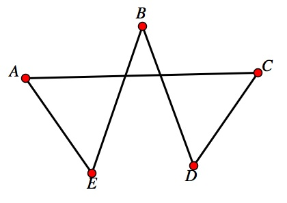 |
b.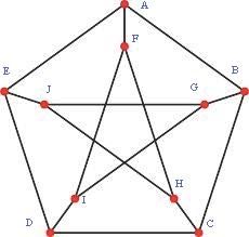 |
c.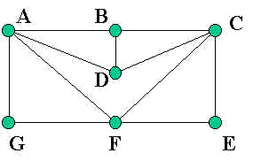 |
Figure \(\PageIndex{1}\): Examples of Hamilton Paths
Not all graphs have a Hamilton circuit or path. There is no way to tell just by looking at a graph if it has a Hamilton circuit or path like you can with an Euler circuit or path. You must do trial and error to determine this. By the way if a graph has a Hamilton circuit then it has a Hamilton path. Just do not go back to home.
Graph a. has a Hamilton circuit (one example is ACDBEA)
Graph b. has no Hamilton circuits, though it has a Hamilton path (one example is ABCDEJGIFH)
Graph c. has a Hamilton circuit (one example is AGFECDBA)
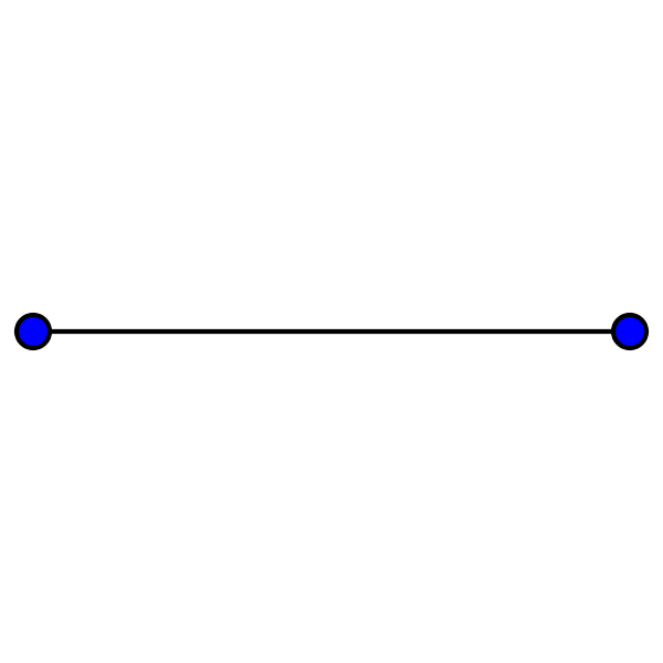
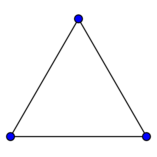
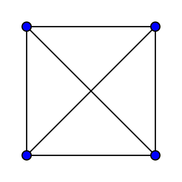
| Complete Graph: A complete graph is a graph with N vertices in which every pair of vertices is joined by exactly one edge. The symbol used to denote a complete graph is KN. |
Example \(\PageIndex{2}\): Complete Graphs
| a. K\(_2\) | b. K\(_3\) | c. K\(_4\) | d. K\(_5\) |
 |
 |
 |
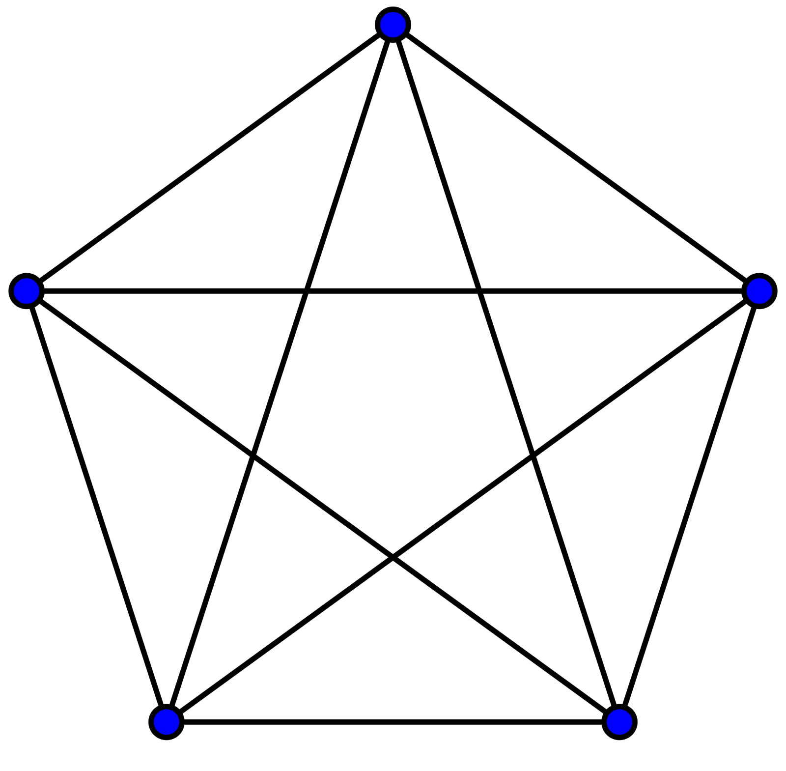 |
| two vertices and one edge | three vertices and three edges | four vertices and six edges | five vertices and ten edges |
Figure \(\PageIndex{2}\): Complete Graphs for N = 2, 3, 4, and 5
In each complete graph shown above, there is exactly one edge connecting each pair of vertices. There are no loops or multiple edges in complete graphs. Complete graphs do have Hamilton circuits.
| Reference Point: the starting point of a Hamilton circuit |
Example \(\PageIndex{3}\): Reference Point in a Complete Graph
Many Hamilton circuits in a complete graph are the same circuit with different starting points. For example, in the graph K3, shown below in Figure \(\PageIndex{3}\), ABCA is the same circuit as BCAB, just with a different starting point (reference point). We will typically assume that the reference point is A.
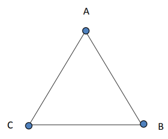
Figure \(\PageIndex{3}\): K\(_3\)
| Number of Hamilton Circuits: A complete graph with N vertices is (N-1)! Hamilton circuits. Since half of the circuits are mirror images of the other half, there are actually only half this many unique circuits. |
Example \(\PageIndex{4}\): Number of Hamilton Circuits
How many Hamilton circuits does a graph with five vertices have?
(N – 1)! = (5 – 1)! = 4! = 4*3*2*1 = 24 Hamilton circuits.
How to solve a Traveling Salesman Problem (TSP):
A traveling salesman problem is a problem where you imagine that a traveling salesman goes on a business trip. He starts in his home city (A) and then needs to travel to several different cities to sell his wares (the other cities are B, C, D, etc.). To solve a TSP, you need to find the cheapest way for the traveling salesman to start at home, A, travel to the other cities, and then return home to A at the end of the trip. This is simply finding the Hamilton circuit in a complete graph that has the smallest overall weight. There are several different algorithms that can be used to solve this type of problem.
A. Brute Force Algorithm
- List all possible Hamilton circuits of the graph.
- For each circuit find its total weight.
- The circuit with the least total weight is the optimal Hamilton circuit.
Example \(\PageIndex{5}\): Brute Force Algorithm:
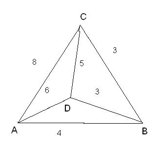
Suppose a delivery person needs to deliver packages to three locations and return to the home office A. Using the graph shown above in Figure \(\PageIndex{4}\), find the shortest route if the weights on the graph represent distance in miles.
Recall the way to find out how many Hamilton circuits this complete graph has. The complete graph above has four vertices, so the number of Hamilton circuits is:
(N – 1)! = (4 – 1)! = 3! = 3*2*1 = 6 Hamilton circuits.
However, three of those Hamilton circuits are the same circuit going the opposite direction (the mirror image).
| Hamilton Circuit | Mirror Image | Total Weight (Miles) |
| ABCDA | ADCBA | 18 |
| ABDCA | ACDBA | 20 |
| ACBDA | ADBCA | 20 |
The solution is ABCDA (or ADCBA) with total weight of 18 mi. This is the optimal solution.
B. Nearest-Neighbor Algorithm:
- Pick a vertex as the starting point.
- From the starting point go to the vertex with an edge with the smallest weight. If there is more than one choice, choose at random.
- Continue building the circuit, one vertex at a time from among the vertices that have not been visited yet.
- From the last vertex, return to the starting point.
Example \(\PageIndex{6}\): Nearest-Neighbor Algorithm
A delivery person needs to deliver packages to four locations and return to the home office A as shown in Figure \(\PageIndex{5}\) below. Find the shortest route if the weights represent distances in miles.
Starting at A, E is the nearest neighbor since it has the least weight, so go to E. From E, B is the nearest neighbor so go to B. From B, C is the nearest neighbor so go to C. From C, the first nearest neighbor is B, but you just came from there. The next nearest neighbor is A, but you do not want to go there yet because that is the starting point. The next nearest neighbor is E, but you already went there. So go to D. From D, go to A since all other vertices have been visited.
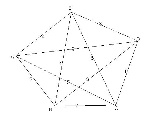
The solution is AEBCDA with a total weight of 26 miles. This is not the optimal solution, but it is close and it was a very efficient method.
C. Repetitive Nearest-Neighbor Algorithm:
- Let X be any vertex. Apply the Nearest-Neighbor Algorithm using X as the starting vertex and calculate the total cost of the circuit obtained.
- Repeat the process using each of the other vertices of the graph as the starting vertex.
- Of the Hamilton circuits obtained, keep the best one. If there is a designated starting vertex, rewrite this circuit with that vertex as the reference point.
Example \(\PageIndex{7}\): Repetitive Nearest-Neighbor Algorithm
Suppose a delivery person needs to deliver packages to four locations and return to the home office A. Find the shortest route if the weights on the graph represent distances in kilometers.
Starting at A, the solution is AEBCDA with total weight of 26 miles as we found in Example \(\PageIndex{6}\). See this solution below in Figure \(\PageIndex{7}\).
Starting at B, the solution is BEDACB with total weight of 20 miles.
Starting at C, the solution is CBEDAC with total weight of 20 miles.
Starting at D, the solution is DEBCAD with total weight of 20 miles.
Starting at E, solution is EBCADE with total weight of 20 miles.
Now, you can compare all of the solutions to see which one has the lowest overall weight. The solution is any of the circuits starting at B, C, D, or E since they all have the same weight of 20 miles. Now that you know the best solution using this method, you can rewrite the circuit starting with any vertex. Since the home office in this example is A, let’s rewrite the solutions starting with A. Thus, the solution is ACBEDA or ADEBCA.
D. Cheapest-Link Algorithm
- Pick the link with the smallest weight first (if there is a tie, randomly pick one). Mark the corresponding edge in red.
- Pick the next cheapest link and mark the corresponding edge in red.
- Continue picking the cheapest link available. Mark the corresponding edge in red except when a) it closes a circuit or b) it results in three edges coming out of a single vertex.
- When there are no more vertices to link, close the red circuit.
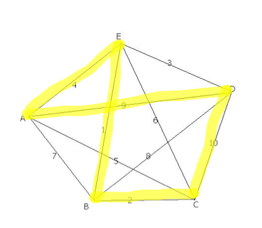
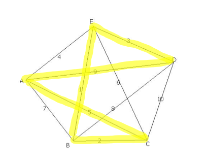
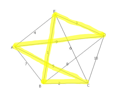
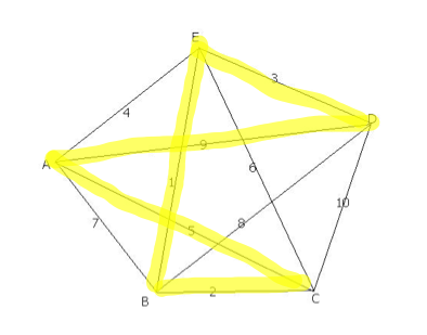
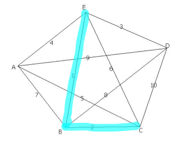
Example \(\PageIndex{8}\): Cheapest-Link Algorithm
Suppose a delivery person needs to deliver packages to four locations and return to the home office A. Find the shortest route if the weights represent distances in miles.
Step 1: Find the cheapest link of the graph and mark it in blue. The cheapest link is between B and E with a weight of one mile.
Step 2: Find the next cheapest link of the graph and mark it in blue. The next cheapest link is between B and C with a weight of two miles.
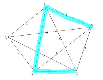
Step 3: Find the next cheapest link of the graph and mark it in blue provided it does not make a circuit or it is not a third edge coming out of a single vertex. The next cheapest link is between D and E with a weight of three miles.
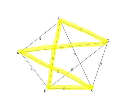
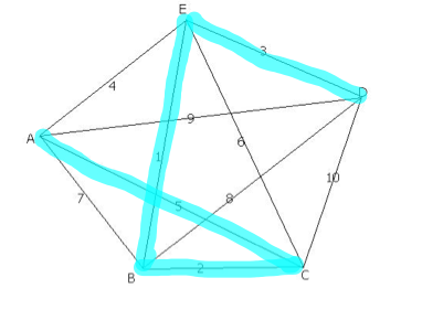
Step 4: Find the next cheapest link of the graph and mark it in blue provided it does not make a circuit or it is not a third edge coming out of a single vertex. The next cheapest link is between A and E with a weight of four miles, but it would be a third edge coming out of a single vertex. The next cheapest link is between A and C with a weight of five miles. Mark it in blue.
Step 5: Since all vertices have been visited, close the circuit with edge DA to get back to the home office, A. This is the only edge we could close the circuit with because AB creates three edges coming out of vertex B and BD also created three edges coming out of vertex B.
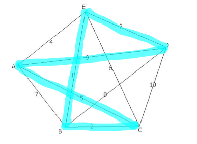
The solution is ACBEDA or ADEBCA with total weight of 20 miles.
| Efficient Algorithm: an algorithm for which the number of steps needed to carry it out grows in proportion to the size of the input to the problem. |
| Approximate Algorithm: any algorithm for which the number of steps needed to carry it out grows in proportion to the size of the input to the problem. There is no known algorithm that is efficient and produces the optimal solution. |