
13.4: Describing Structural Equivalence Sets

( \newcommand{\kernel}{\mathrm{null}\,}\)
Two actors that are structurally equivalent have the same ties to all other actors - they are perfectly substitutable or exchangeable. In "real" data, exact equivalence may be quite rare, and it many be meaningful to measure approximate equivalence. There are several approaches for examining the pattern of similarities in the tie-profiles of actors, and for forming structural equivalence classes.
One very useful approach is to apply cluster analysis to attempt to discern how many structural equivalence sets there are, and which actors fall within each set. We will examine two more common approaches - CONCOR, and numerical optimization by tabu search.
What the similarity matrix and cluster analysis do not tell us is what similarities make the actors in each set "the same" and which differences make the actors in one set "different" from the actors in another. A very useful approach to understanding the bases of similarity and difference among sets of structurally equivalent actors is the block model, and a summary based on it called the image matrix. Both of these ideas have been explained elsewhere. We will take a look at how they can help us to understand the results of CONCOR and tabu search.
Clustering Similarities or Distances Profiles
Cluster analysis is a natural method for exploring structural equivalence. Two actors who have the similar patterns of ties to other actors will be joined into a cluster, and hierarchical methods will show a "tree" of successive joining.
Network>Roles & Positions>Structural>Profile can perform a variety of kinds of cluster analysis for assessing structural equivalence. Figure 13.12 shows a typical dialog for this algorithm.
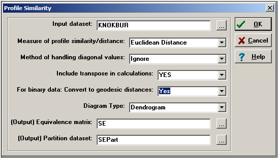
Figure 13.12: Dialog of Network>Roles & Positions>Structural>Profile
Depending on how the relations between actors have been measured, several common ways of constructing the actor-by-actor similarity or distance matrix are provided (correlations, Euclidean distances, total matches, or Jaccard coefficients). Should you desire a different measure of similarity, you can construct it elsewhere (e.g. Tools>Similarities), save the result, and apply cluster analysis directly (i.e. Tools>Cluster).
There are some other important choices. One is, what to do with the items in the similarity matrix that index the similarity of an actor to themselves (i.e. the diagonal values)? One choice ("Retain") includes the similarity of a node with itself; another choice ("Ignore") excludes diagonal elements from the calculation of similarity or difference. The default method ("Reciprocal") replaces the diagonal element for both cases with the tie that exists between the cases.
One may "Include transpose" or not. If the data being examined are symmetric (i.e. a simple graph, not a directed one), then the transpose is identical to the matrix, and shouldn't be included. For directed data, the algorithm will, by default, calculate similarities on the rows (out-ties) but not in-ties. If you want to include the full profile of both in and out ties for directed data, you need to include the transpose.
If you are working with a raw adjacency matrix, similarity can be computed on the tie profile (probably using a match or Jaccard approach). Alternatively, the adjacencies can be turned into a valued measure of dissimilarity by calculating geodesic distances (in which case correlations or Euclidean distances might be chosen as a measure of similarity).
Figure 13.13 shows the results of the analysis described in the dialog.
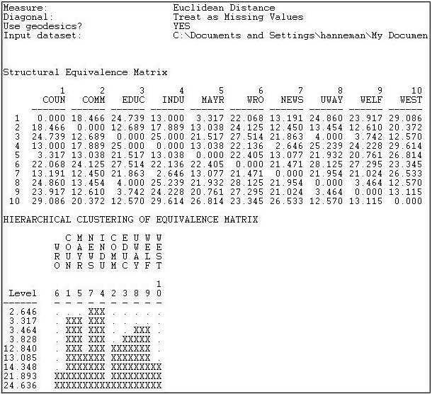
Figure 13.13: Profile similarity of geodesic distances of rows and columns of Knoke information network
The first panel shows the structural equivalence matrix - or the degree of similarity among pairs of actors (in this case, dissimilarity, since we chose to analyze Euclidean distances).
The second panel shows a rough character-mapped graphic of the clustering. Here we see that actors 7 and 4 are most similar, a second cluster is formed by actors 1 and 5; a third by actors 8 and 9. This algorithm also provides a more polished presentation of the result as a dendogram in a separate window, as shown in Figure 13.14.
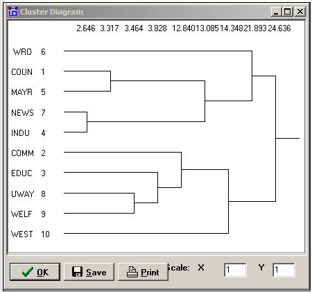
Figure 13.14: Dendogram of structural equivalence data (see Figure 13.13)
There are no exact structural equivalence in the example data. That is, there are no two cases that have identical ties to all other cases. The dendogram can be particularly helpful in locating groupings of cases that are sufficiently equivalent to be treated as classes. The measures of clustering adequacy in Tools>Cluster can provide additional guidance.
Two other approaches, CONCOR and optimization, follow a somewhat different logic than clustering. In both of these methods, partitions or approximate equivalence classes are set up first (the user selects how many), and the cases are allocated to these classes by numerical techniques designed to maximize similarity within classes.
CONCOR
CONCOR is an approach that has been used for quite some time. Although the algorithm of CONCOR is now regarded as a bit peculiar, the technique usually produces meaningful results.
CONCOR begins by correlating each pair of actors (as we did above). Each row of this actor-by-actor correlation matrix is then extracted, and correlated with each other row. In a sense, the approach is asking "how similar is the vector of similarities of actor X to the vector of similarities of actor Y"? This process is repeated over and over. Eventually the elements in this "iterated correlation matrix" converge on a value of either +1 or -1 (if you want to convince yourself, give it a try!).
CONCOR then divides the data into two sets on the basis of these correlations. Then, within each set (if it has more than two actors) the process is repeated. The process continues until all actors are separated (or until we lose interest). The result is a binary branching tree that gives rise to a final partition.
For illustration, we have asked CONCOR to show us the groups that best satisfy this property when we believe that there are four groups in the Knoke information data. We used Network>Roles & Positions>Structural>CONCOR, and set the depth of splits = 2 (that is, divide the data twice). All blocking algorithms require that we have a prior idea about how many groups there are. The results are shown in Figure 13.15.
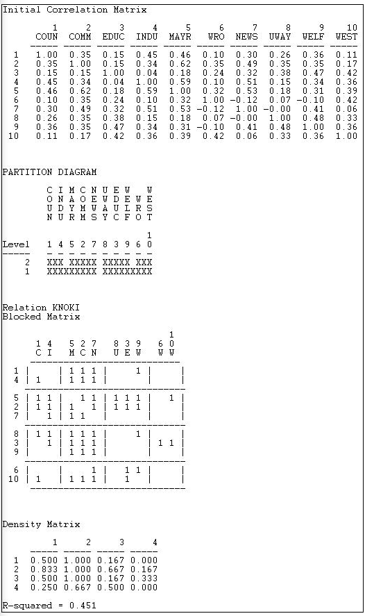
Figure 13.15: CONCOR on Knoke information matrix with two splits
The first panel shows the correlations of the cases. We included the transpose, so these correlations are based on both sending and receiving of ties. Our data, however, are binary, so the use of the correlation coefficient (and CONCOR) should be treated with caution.
The second panel shows the two splits. In the first division, the two groups {1, 4, 5, 2, 7} and {8, 3, 9, 6, 10} were formed. On the second split these were sub-divided into {1, 4}, {5, 2, 7}, {8, 3, 9}, and {6, 10}.
The third panel (the "Blocked Matrix") shows the permuted original data. The result here could be simplified further by creating a "block image" matrix of the four classes by the four classes, with "1" in high density blocks and "0" in low density blocks - as in Figure 13.16.
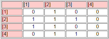
Figure 13.16: Block image of CONCOR results
The goodness of fit of a block model can be assessed by correlating the permuted matrix (the block model) against a "perfect" model with the same blocks (i.e. one in which all elements of one blocks are ones, and all elements of zero blocks are zeros). For the CONCOR two-split (four group) model, this r-squared is 0.451. That is, about 1/2 of the variance in the ties in the CONCOR model can be accounted for by a "perfect" structural block model. This might be regarded as OK, but is hardly a wonderful fit (there is no real criterion for what is a good fit).
The block model and its image also provide a description of what it means when we say "the actors in block one are approximately structurally equivalent". Actors in equivalence class one are likely to send ties to all other actors in block two, but no other block. Actors in equivalence class one are likely to receive ties from all actors in blocks 2 and 3. So, we have not only identified the classes, we've also described the form of the relations that makes the cases equivalent.
Optimization by Tabu Search
This method of blocking has been developed more recently, and relies on extensive use of the computer. Tabu search uses a more modern (and computer intensive) algorithm than CONCOR, but is trying to implement the same idea of grouping together actors who are most similar into a block. Tabu search does this by searching for sets of actors who, if placed into a block, produce the smallest sum of within-block variances in the tie profiles. That is, if actors in a block have similar ties, their variance around the block mean profile will be small. So, the partitioning that minimizes the sum of within block variances is minimizing the overall variance in tie profiles. In principle, this method ought to produce results similar (but not necessarily identical) to CONCOR. In practice, this is not always so. Here (Figure 13.17) are the results of Network>Roles & Positions>Structural>Optimization>Binary applied to the Knoke information network, and requesting four classes. A variation of the technique for valued data is available as Network>Roles & Positions>Structural>Optimization>Valued.
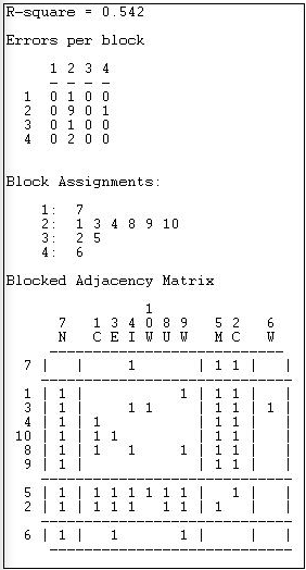
Figure 13.17: Optimized four-block solution for structural equivalence of Knoke information network
The overall correlation between the actual scores in the blocked matrix, and a "perfect" matrix composed of only ones and zeros is reasonably good (0.544).
The suggested partition into structural equivalence classes is {7}, {1, 3, 4, 10, 8, 9}, {5, 2}, and {6}.
We can now also describe the positions of each of the classes. The first class (actor 7) has dense sending ties to the third (actors 5 and 2); and receives information from all three other classes. The second, and largest, class sends information to the first and the third class, and receives information from the third class. The last class (actor 6), sends to the first class, but receives from none.
This last analysis illustrates most fully the primary goals of an analysis of structural equivalence:
1) How many equivalence classes, or approximate equivalence classes, are there?
2) How good is the fit of this simplification into equivalence classes in summarizing the information about all the nodes?
3) What is the position of each class, as defined by its relations to the other classes?