5.6: Graphing Linear Equations and Inequalities
- Page ID
- 129557

\( \newcommand{\vecs}[1]{\overset { \scriptstyle \rightharpoonup} {\mathbf{#1}} } \)
\( \newcommand{\vecd}[1]{\overset{-\!-\!\rightharpoonup}{\vphantom{a}\smash {#1}}} \)
\( \newcommand{\id}{\mathrm{id}}\) \( \newcommand{\Span}{\mathrm{span}}\)
( \newcommand{\kernel}{\mathrm{null}\,}\) \( \newcommand{\range}{\mathrm{range}\,}\)
\( \newcommand{\RealPart}{\mathrm{Re}}\) \( \newcommand{\ImaginaryPart}{\mathrm{Im}}\)
\( \newcommand{\Argument}{\mathrm{Arg}}\) \( \newcommand{\norm}[1]{\| #1 \|}\)
\( \newcommand{\inner}[2]{\langle #1, #2 \rangle}\)
\( \newcommand{\Span}{\mathrm{span}}\)
\( \newcommand{\id}{\mathrm{id}}\)
\( \newcommand{\Span}{\mathrm{span}}\)
\( \newcommand{\kernel}{\mathrm{null}\,}\)
\( \newcommand{\range}{\mathrm{range}\,}\)
\( \newcommand{\RealPart}{\mathrm{Re}}\)
\( \newcommand{\ImaginaryPart}{\mathrm{Im}}\)
\( \newcommand{\Argument}{\mathrm{Arg}}\)
\( \newcommand{\norm}[1]{\| #1 \|}\)
\( \newcommand{\inner}[2]{\langle #1, #2 \rangle}\)
\( \newcommand{\Span}{\mathrm{span}}\) \( \newcommand{\AA}{\unicode[.8,0]{x212B}}\)
\( \newcommand{\vectorA}[1]{\vec{#1}} % arrow\)
\( \newcommand{\vectorAt}[1]{\vec{\text{#1}}} % arrow\)
\( \newcommand{\vectorB}[1]{\overset { \scriptstyle \rightharpoonup} {\mathbf{#1}} } \)
\( \newcommand{\vectorC}[1]{\textbf{#1}} \)
\( \newcommand{\vectorD}[1]{\overrightarrow{#1}} \)
\( \newcommand{\vectorDt}[1]{\overrightarrow{\text{#1}}} \)
\( \newcommand{\vectE}[1]{\overset{-\!-\!\rightharpoonup}{\vphantom{a}\smash{\mathbf {#1}}}} \)
\( \newcommand{\vecs}[1]{\overset { \scriptstyle \rightharpoonup} {\mathbf{#1}} } \)
\( \newcommand{\vecd}[1]{\overset{-\!-\!\rightharpoonup}{\vphantom{a}\smash {#1}}} \)
\(\newcommand{\avec}{\mathbf a}\) \(\newcommand{\bvec}{\mathbf b}\) \(\newcommand{\cvec}{\mathbf c}\) \(\newcommand{\dvec}{\mathbf d}\) \(\newcommand{\dtil}{\widetilde{\mathbf d}}\) \(\newcommand{\evec}{\mathbf e}\) \(\newcommand{\fvec}{\mathbf f}\) \(\newcommand{\nvec}{\mathbf n}\) \(\newcommand{\pvec}{\mathbf p}\) \(\newcommand{\qvec}{\mathbf q}\) \(\newcommand{\svec}{\mathbf s}\) \(\newcommand{\tvec}{\mathbf t}\) \(\newcommand{\uvec}{\mathbf u}\) \(\newcommand{\vvec}{\mathbf v}\) \(\newcommand{\wvec}{\mathbf w}\) \(\newcommand{\xvec}{\mathbf x}\) \(\newcommand{\yvec}{\mathbf y}\) \(\newcommand{\zvec}{\mathbf z}\) \(\newcommand{\rvec}{\mathbf r}\) \(\newcommand{\mvec}{\mathbf m}\) \(\newcommand{\zerovec}{\mathbf 0}\) \(\newcommand{\onevec}{\mathbf 1}\) \(\newcommand{\real}{\mathbb R}\) \(\newcommand{\twovec}[2]{\left[\begin{array}{r}#1 \\ #2 \end{array}\right]}\) \(\newcommand{\ctwovec}[2]{\left[\begin{array}{c}#1 \\ #2 \end{array}\right]}\) \(\newcommand{\threevec}[3]{\left[\begin{array}{r}#1 \\ #2 \\ #3 \end{array}\right]}\) \(\newcommand{\cthreevec}[3]{\left[\begin{array}{c}#1 \\ #2 \\ #3 \end{array}\right]}\) \(\newcommand{\fourvec}[4]{\left[\begin{array}{r}#1 \\ #2 \\ #3 \\ #4 \end{array}\right]}\) \(\newcommand{\cfourvec}[4]{\left[\begin{array}{c}#1 \\ #2 \\ #3 \\ #4 \end{array}\right]}\) \(\newcommand{\fivevec}[5]{\left[\begin{array}{r}#1 \\ #2 \\ #3 \\ #4 \\ #5 \\ \end{array}\right]}\) \(\newcommand{\cfivevec}[5]{\left[\begin{array}{c}#1 \\ #2 \\ #3 \\ #4 \\ #5 \\ \end{array}\right]}\) \(\newcommand{\mattwo}[4]{\left[\begin{array}{rr}#1 \amp #2 \\ #3 \amp #4 \\ \end{array}\right]}\) \(\newcommand{\laspan}[1]{\text{Span}\{#1\}}\) \(\newcommand{\bcal}{\cal B}\) \(\newcommand{\ccal}{\cal C}\) \(\newcommand{\scal}{\cal S}\) \(\newcommand{\wcal}{\cal W}\) \(\newcommand{\ecal}{\cal E}\) \(\newcommand{\coords}[2]{\left\{#1\right\}_{#2}}\) \(\newcommand{\gray}[1]{\color{gray}{#1}}\) \(\newcommand{\lgray}[1]{\color{lightgray}{#1}}\) \(\newcommand{\rank}{\operatorname{rank}}\) \(\newcommand{\row}{\text{Row}}\) \(\newcommand{\col}{\text{Col}}\) \(\renewcommand{\row}{\text{Row}}\) \(\newcommand{\nul}{\text{Nul}}\) \(\newcommand{\var}{\text{Var}}\) \(\newcommand{\corr}{\text{corr}}\) \(\newcommand{\len}[1]{\left|#1\right|}\) \(\newcommand{\bbar}{\overline{\bvec}}\) \(\newcommand{\bhat}{\widehat{\bvec}}\) \(\newcommand{\bperp}{\bvec^\perp}\) \(\newcommand{\xhat}{\widehat{\xvec}}\) \(\newcommand{\vhat}{\widehat{\vvec}}\) \(\newcommand{\uhat}{\widehat{\uvec}}\) \(\newcommand{\what}{\widehat{\wvec}}\) \(\newcommand{\Sighat}{\widehat{\Sigma}}\) \(\newcommand{\lt}{<}\) \(\newcommand{\gt}{>}\) \(\newcommand{\amp}{&}\) \(\definecolor{fillinmathshade}{gray}{0.9}\)Learning Objectives
After completing this section, you should be able to:
- Graph linear equations and inequalities in two variables.
- Solve applications of linear equations and inequalities.
In this section, we will learn how to graph linear equations and inequalities. There are several real-world scenarios that can be represented by graphs of linear inequalities. Think of filling your car up with gasoline. If gasoline is $3.99 per gallon and you put 10 gallons in your car, you will pay $39.90. Your friend buys 15 gallons of gasoline and pays $59.85. You can plot these points on a coordinate system and connect the points with a line to create the graph of a line. You'll learn to do both in this section.
Plotting Points on a Rectangular Coordinate System
Just like maps use a grid system to identify locations, a grid system is used in algebra to show a relationship between two variables in a rectangular coordinate system. The rectangular coordinate system is also called the -plane or the “coordinate plane.”
The rectangular coordinate system is formed by two intersecting number lines, one horizontal and one vertical. The horizontal number line is called the
In the rectangular coordinate system, every point is represented by an ordered pair (Figure 5.21). The first number in the ordered pair is the -coordinate of the point, and the second number is the -coordinate of the point. The phrase "ordered pair" means that the order is important. At the point where the axes cross and where both coordinates are zero, the ordered pair is . The point has a special name. It is called the origin.
We use the coordinates to locate a point on the
Notice that the vertical line through
Example 5.39
Plotting Points on a Coordinate System
Plot the following points in the rectangular coordinate system and identify the quadrant in which the point is located:
- Answer
The first number of the coordinate pair is the
- Since , the point is to the left of the -axis. Also, since , the point is above the -axis. The point is in quadrant II.
- Since , the point is to the left of the -axis. Also, since , the point is below the -axis. The point is in quadrant III.
- Since , the point is to the right of the -axis. Since , the point is below the -axis. The point is in quadrant IV.
- Since , the point whose coordinates are is on the -axis.
- Since , the point is to the right of the -axis. Since , which is equal to 2.5, the point is above the -axis. The point is in quadrant I.
Figure 5.24
Your Turn 5.39
- /**/\left( { - 4,2} \right)/**/
- /**/ (–1, –2)/**/
- /**/ (3, –5)/**/
- /**/\left(–3,0 \right)/**/
- /**/ (\frac{5}{3},2)/**/
Graphing Linear Equations in Two Variables
Up to now, all the equations you have solved were equations with just one variable. In almost every case, when you solved the equation, you got exactly one solution. But equations can have more than one variable. Equations with two variables may be of the form . An equation of this form, where and are both not zero, is called a linear equation in two variables. Here is an example of a linear equation in two variables, and .
The equation is also a linear equation. But it does not appear to be in the form . We can use the addition property of equality and rewrite it in form.
Step 1: Add to both sides.
Step 2: Simplify.
Step 3: Put it in form.
By rewriting as , we can easily see that it is a linear equation in two variables because it is of the form . When an equation is in the form , we say it is in standard form of a linear equation. Most people prefer to have , , and be integers and when writing a linear equation in standard form, although it is not strictly necessary.
Linear equations have infinitely many solutions. For every number that is substituted for there is a corresponding value. This pair of values is a solution to the linear equation and is represented by the ordered pair (,). When we substitute these values of and into the equation, the result is a true statement, because the value on the left side is equal to the value on the right side.
We can plot these solutions in the rectangular coordinate system. The points will line up perfectly in a straight line. We connect the points with a straight line to get the graph of the linear equation. We put arrows on the ends of each side of the line to indicate that the line continues in both directions.
A graph is a visual representation of all the solutions of a linear equation. The line shows you all the solutions to that linear equation. Every point on the line is a solution of that linear equation. And every solution of the linear equation is on this line. This line is called the graph of the equation. Points not on the line are not solutions! The graph of a linear equation is a straight line.
- Every point on the line is a solution of the equation.
- Every solution of this equation is a point on this line.
Example 5.40
Determining Points on a Line
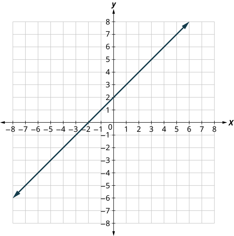
Figure 5.25 is the graph of .
For each ordered pair, decide:
- Is the ordered pair a solution to the equation?
- Is the point on the line?
- Answer
Substitute the - and -values into the equation to check if the ordered pair is a solution to the equation.
- Plot the points , , , and .
Figure 5.26In Figure 5.26, the points , , and are on the line , and the point is not on the line. The points that are solutions to are on the line, but the point that is not a solution is not on the line.
Your Turn 5.40
- Is the ordered pair a solution to the equation?
- Is the point on the line?
The steps to take when graphing a linear equation by plotting points are:
Step 1: Find three points whose coordinates are solutions to the equation. Organize them in a table.
Step 2: Plot the points in a rectangular coordinate system. Check that the points line up. If they do not, carefully check your work.
Step 3: Draw the line through the three points. Extend the line to fill the grid and put arrows on both ends of the line.
It is true that it only takes two points to determine a line, but it is a good habit to use three points. If you only plot two points and one of them is incorrect, you can still draw a line, but it will not represent the solutions to the equation. It will be the wrong line. If you use three points, and one is incorrect, the points will not line up. This tells you something is wrong, and you need to check your work.
Example 5.41
Graphing a Line by Plotting Points
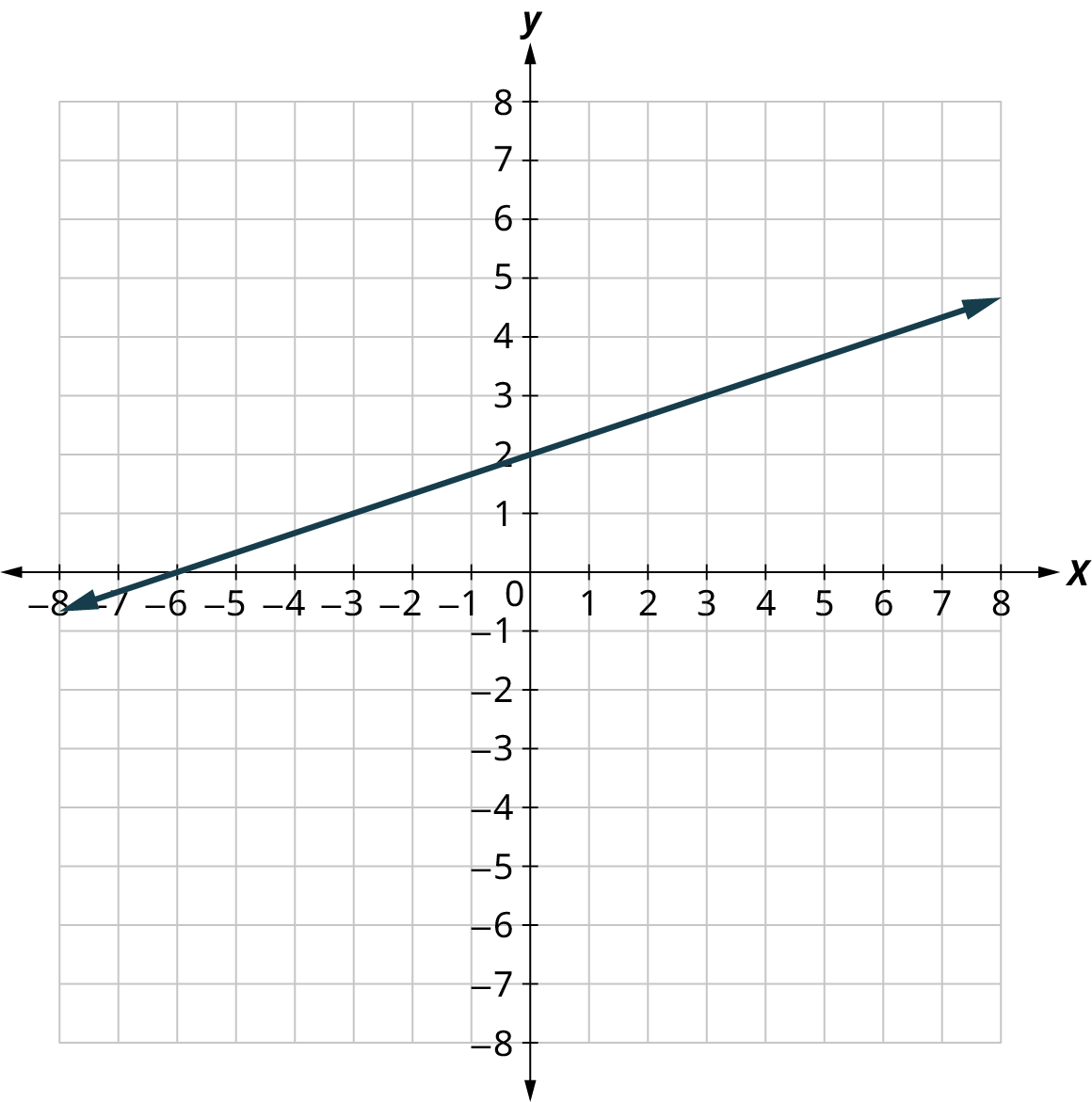
Graph the equation: .
- Answer
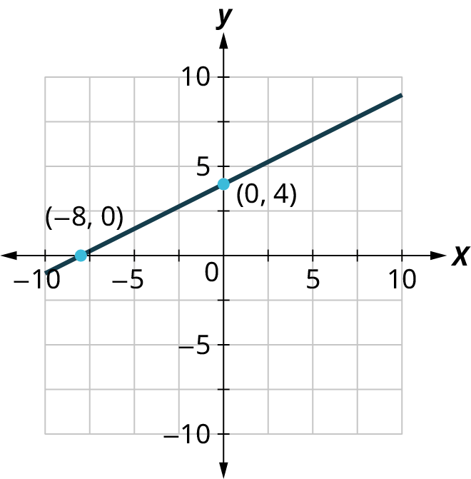
Find three points that are solutions to the equation. Since this equation has the fraction as a coefficient of , we will choose values of carefully. We will use zero as one choice and multiples of 2 for the other choices. Why are multiples of two a good choice for values of ? By choosing multiples of 2, the multiplication by simplifies to a whole number.
(, ) 0 3 2 4 4 5 Plot the points, check that they line up, and draw the line (Figure 5.28).
Figure 5.28
Your Turn 5.41
Solving Applications Using Linear Equations in Two Variables
Many fields use linear equalities to model a problem. While our examples may be about simple situations, they give us an opportunity to build our skills and to get a feel for how they might be used.
Example 5.42
Pumping Gas
Gasoline costs $3.53 per gallon. You put 10 gallons of gasoline in your car, and pay $35.30. Your friend puts 15 gallons of gasoline in their car and pays $52.95. Your neighbor needs 5 gallons of gasoline, how much will they pay?
- Answer
Let
Figure 5.29
We can see the point at . The -value is found by multiplying 5 by $3.53 to get $17.65. Your neighbor will pay $17.65.
Your Turn 5.42
People in Mathematics
René Descartes
René Descartes was born in 1596 in La Haye, France. He was sickly as a child, so much so that he was allowed to stay in bed until 11:00 AM rather than get up at 5:00 AM like the other school children. He kept this habit of rising late for most of the rest of his life.
After his primary schooling, Descartes attended the University of Poitiers, receiving a law degree in 1616. He then embarked on a myriad of journeys, joining two different militaries (one in the Netherlands, the other in Bavaria) and generally travelling around Europe until 1628, when he settled in the Netherlands. It was here that he began to delve deeply into his ideas of science, mathematics, and philosophy.
In 1637, at the urging of his friends, Descartes published Discourse on the Method for Conducting One's Reason Well and Seeking the Truth in the Sciences. The book had three appendices: La Dioptrique, a work on optics; Les Météores, which pertained to meteorology; and La Géométrie, a work on mathematics. It was in this appendix that he proposed a geometric way of representing many different algebraic expressions and equations. It is this system of representation that almost all mathematical textbooks use today.
These publications (along with several others) brought much fame to Descartes. So renowned was his reputation that late in 1649, Queen Christina of Sweden asked Descartes to come to Sweden to tutor her. However, she wished to do her studies at 5:00 in the morning; Descartes had to break his lifelong habit of sleeping in late. A few months later, in February 1650, Descartes died of pneumonia.
Graphing Linear Inequalities
Previously we learned to solve inequalities with only one variable. We will now learn about inequalities containing two variables that can be written in one of the following forms: , , , and where and are not both zero. We will look at linear inequalities in two variables, which are very similar to linear equations in two variables.
Like linear equations, linear inequalities in two variables have many solutions. Any ordered pair (, ) that makes an inequality true when we substitute in the values is a solution to a linear inequality.
Example 5.43
Determining Solutions to an Inequality
Determine whether each ordered pair is a solution to the inequality :
- Answer
Your Turn 5.43
Let us think about
Similarly, the line separates the plane into two regions. On one side of the line are points with . On the other side of the line are the points with . We call the line a boundary line.
For an inequality in one variable, the endpoint is shown with a parenthesis (Figure 5.32) or a bracket (Figure 5.33) depending on whether or not is included in the solution:
Similarly, for an inequality in two variables, the boundary line is shown with a solid or dashed line to show whether or not it the line is included in the solution.
| Boundary line is | Boundary line is |
| Boundary line is not included in solution. | Boundary line is included in solution. |
| Boundary line is dashed. | Boundary line is solid. |
Now, let us take a look at what we found in Example 5.43. We will start by graphing the line
Let us take another point above the boundary line and test whether or not it is a solution to the inequality . The point clearly looks to be above the boundary line, doesn’t it? Is it a solution to the inequality?
Yes,
The graph of the inequality
Example 5.44
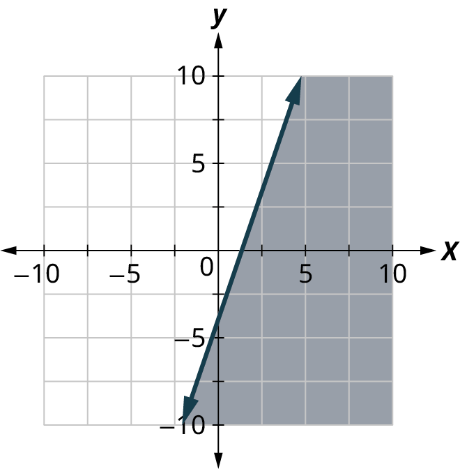
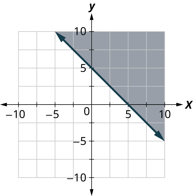
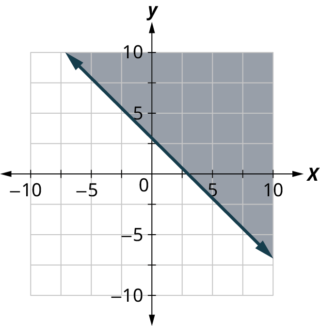
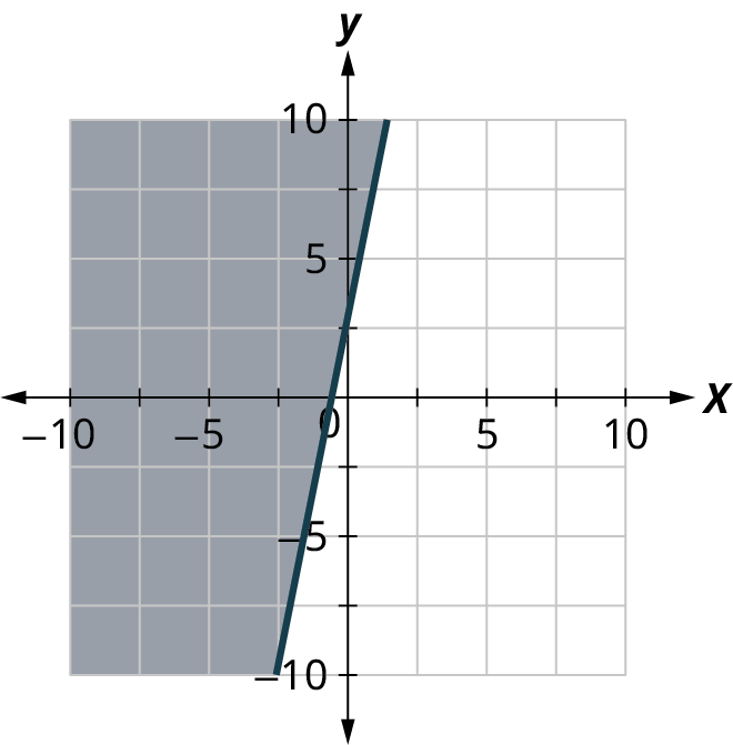
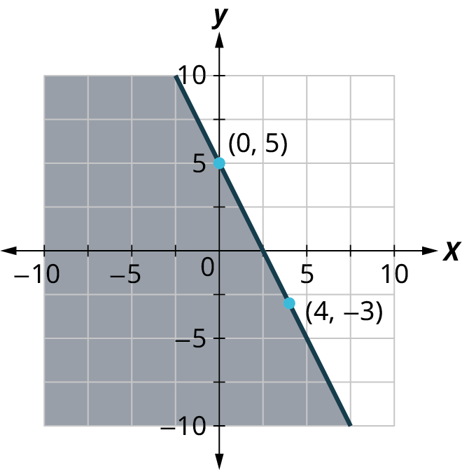
Writing a Linear Inequality Shown by a Graph
The boundary line shown in this graph is
- Answer
The line is the boundary line. On one side of the line are the points with and on the other side of the line are the points with . Let us test the point and see which inequality describes its position relative to the boundary line. At , which inequality is true: or ?
True False Since is true, the side of the line with , is the solution. The shaded region shows the solution of the inequality . Since the boundary line is graphed with a dashed line, the inequality does not include the equal sign. The graph shows the inequality .
We could use an point as a test point, provided it is not on the line. Why did we choose ? Because it is the easiest to evaluate. You may want to pick a point on the other side of the boundary line and check that .
Your Turn 5.44
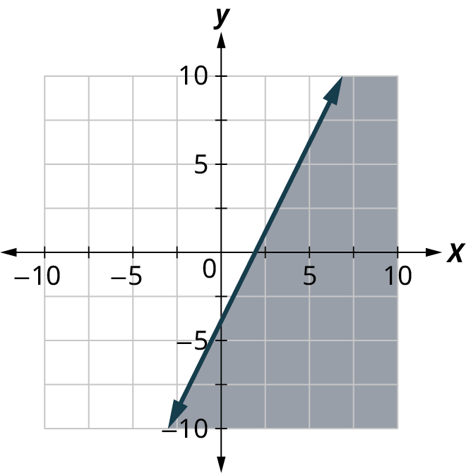
Example 5.45
Graphing a Linear Inequality
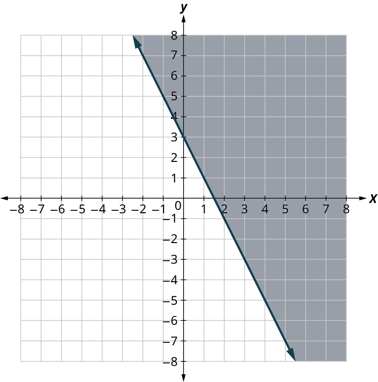
Graph the linear inequality .
- Answer
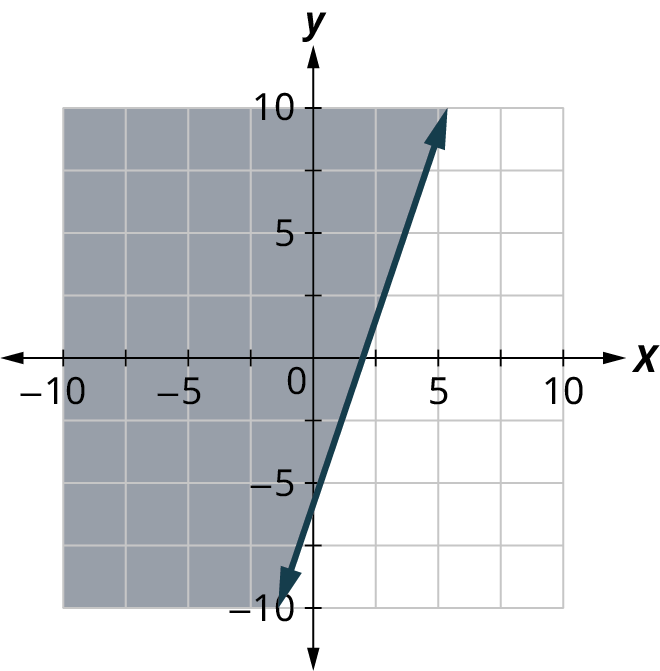
Step 1. Identify and graph the boundary line (Figure 5.38).
- If the inequality is ≤ or ≥, the boundary line is solid.
- If the inequality is < or >, the boundary line is dashed.
Replace the inequality sign with an equal sign to find the boundary line.
Graph the boundary line .
The inequality sign is ≥, so we draw a solid line.
Figure 5.38
We’ll test .
Is it a solution of the inequality?
At , is ?
So, is a solution.
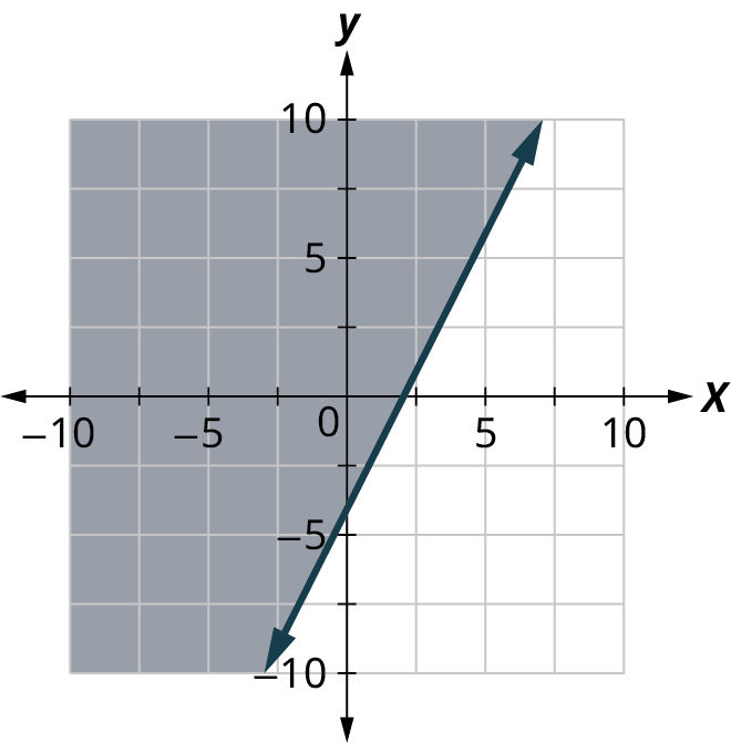
Step 3. Shade in one side of the boundary line (Figure 5.39).
- If the test point is a solution, shade in the side that includes the point.
- If the test point is not a solution, shade in the opposite side.
All points in the shaded region and on the boundary line represent the solution to .
Your Turn 5.45
Video
Solving Applications Using Linear Inequalities in Two Variables
Many fields use linear inequalities to model a problem. While our examples may be about simple situations, they give us an opportunity to build our skills and to get a feel for how they might be used.
Example 5.46
Working Multiple Jobs
Hilaria works two part time jobs to earn enough money to meet her obligations of at least $240 a week. Her job in food service pays $10 an hour and her tutoring job on campus pays $15 an hour. How many hours does Hilaria need to work at each job to earn at least $240?
- Let be the number of hours she works at the job in food service and let be the number of hours she works tutoring. Write an inequality that would model this situation.
- Graph the inequality.
- Find three ordered pairs () that would be solutions to the inequality. Then, explain what that means for Hilaria.
- Answer
- Let be the number of hours she works at the job in food service and let be the number of hours she works tutoring. She earns $10 per hour at the job in food service and $15 an hour tutoring. At each job, the number of hours multiplied by the hourly wage will give the amount earned at that job.
- Graph the inequality:
Step 1: Graph the boundary line
Create a table of values
0 6 12 Step 2: Pick a test point. Let us pick again:
?
Figure 5.40
For Hilaria, it means that to earn at least $240, she can work 15 hours tutoring and 10 hours at her food service job, earn all her money tutoring for 16 hours, or earn all her money while working 24 hours at the job in food service.
Your Turn 5.46
Check Your Understanding
-
/**/y = 5/**/
-
/**/y = -1/**/
-
/**/y = \frac{1}{2}/**/
-
/**/y = \frac{5}{3}/**/
-
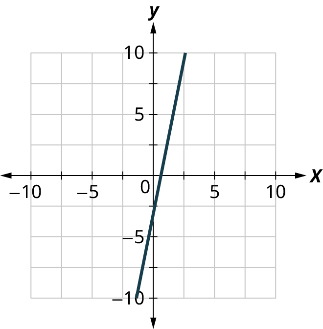
/**/y = 2x + 4/**/
-
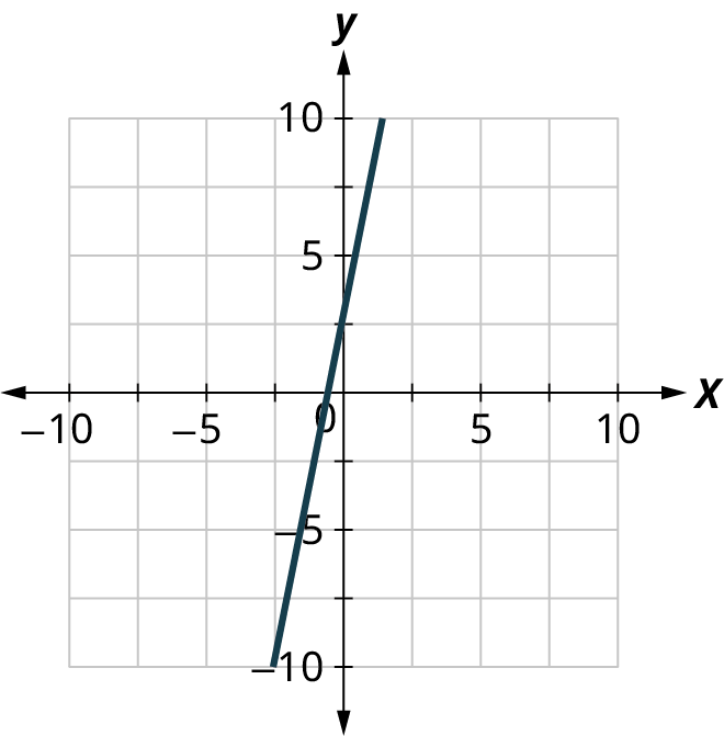
/**/y = \frac{1}{2}x + 4/**/
-
/**/y = - 2x + 4/**/
-
/**/y = \frac{1}{2}x + 4/**/


-
/**/y = -2x + 5/**/
-
/**/y \leq -2x + 5/**/
-
/**/y \geq -2x + 5/**/
-
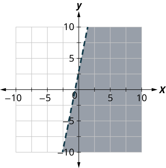
/**/y < -2x + 5/**/
Section 5.5 Exercises
- /**/(3, -1)/**/
- /**/(-3, 1)/**/
- /**/(-2, 0)/**/
- /**/(-4, -3)/**/
- /**/(1,\frac14{5})/**/
- Is the ordered pair a solution to the equation?
- Is the point on the line in the given graph?
- Is the ordered pair a solution to the equation?
- Is the point on the line in the given graph?
- Is the ordered pair a solution to the equation?
- Is the point on the line in the given graph?
/**/{\text{A: (0, 0)}}\quad\quad
Callstack:
    at (Bookshelves/Applied_Mathematics/Contemporary_Mathematics_(OpenStax)/05:__Algebra/5.06:__Graphing_Linear_Equations_and_Inequalities), /content/body/div[5]/div[5]/div/div[12]/div[3]/div[26]/div[2]/div/span[2]/span[1], line 1, column 1
Callstack:
    at (Bookshelves/Applied_Mathematics/Contemporary_Mathematics_(OpenStax)/05:__Algebra/5.06:__Graphing_Linear_Equations_and_Inequalities), /content/body/div[5]/div[5]/div/div[12]/div[3]/div[26]/div[2]/div/span[2]/span[2], line 1, column 1
Callstack:
    at (Bookshelves/Applied_Mathematics/Contemporary_Mathematics_(OpenStax)/05:__Algebra/5.06:__Graphing_Linear_Equations_and_Inequalities), /content/body/div[5]/div[5]/div/div[12]/div[3]/div[26]/div[2]/div/span[2]/span[3], line 1, column 1
Callstack:
    at (Bookshelves/Applied_Mathematics/Contemporary_Mathematics_(OpenStax)/05:__Algebra/5.06:__Graphing_Linear_Equations_and_Inequalities), /content/body/div[5]/div[5]/div/div[12]/div[3]/div[26]/div[2]/div/span[2]/span[4], line 1, column 1
/**/{\text{A: (0, 3)}}\quad\quad
Callstack:
    at (Bookshelves/Applied_Mathematics/Contemporary_Mathematics_(OpenStax)/05:__Algebra/5.06:__Graphing_Linear_Equations_and_Inequalities), /content/body/div[5]/div[5]/div/div[12]/div[3]/div[27]/div/span[2]/span[1], line 1, column 1
Callstack:
    at (Bookshelves/Applied_Mathematics/Contemporary_Mathematics_(OpenStax)/05:__Algebra/5.06:__Graphing_Linear_Equations_and_Inequalities), /content/body/div[5]/div[5]/div/div[12]/div[3]/div[27]/div/span[2]/span[2], line 1, column 1
Callstack:
    at (Bookshelves/Applied_Mathematics/Contemporary_Mathematics_(OpenStax)/05:__Algebra/5.06:__Graphing_Linear_Equations_and_Inequalities), /content/body/div[5]/div[5]/div/div[12]/div[3]/div[27]/div/span[2]/span[3], line 1, column 1
Callstack:
    at (Bookshelves/Applied_Mathematics/Contemporary_Mathematics_(OpenStax)/05:__Algebra/5.06:__Graphing_Linear_Equations_and_Inequalities), /content/body/div[5]/div[5]/div/div[12]/div[3]/div[27]/div/span[2]/span[4], line 1, column 1
/**/{\text{A: (-3, 0)}}\quad\quad
Callstack:
    at (Bookshelves/Applied_Mathematics/Contemporary_Mathematics_(OpenStax)/05:__Algebra/5.06:__Graphing_Linear_Equations_and_Inequalities), /content/body/div[5]/div[5]/div/div[12]/div[3]/div[28]/div/span[2]/span[1], line 1, column 1
Callstack:
    at (Bookshelves/Applied_Mathematics/Contemporary_Mathematics_(OpenStax)/05:__Algebra/5.06:__Graphing_Linear_Equations_and_Inequalities), /content/body/div[5]/div[5]/div/div[12]/div[3]/div[28]/div/span[2]/span[2], line 1, column 1
Callstack:
    at (Bookshelves/Applied_Mathematics/Contemporary_Mathematics_(OpenStax)/05:__Algebra/5.06:__Graphing_Linear_Equations_and_Inequalities), /content/body/div[5]/div[5]/div/div[12]/div[3]/div[28]/div/span[2]/span[3], line 1, column 1
Callstack:
    at (Bookshelves/Applied_Mathematics/Contemporary_Mathematics_(OpenStax)/05:__Algebra/5.06:__Graphing_Linear_Equations_and_Inequalities), /content/body/div[5]/div[5]/div/div[12]/div[3]/div[28]/div/span[2]/span[4], line 1, column 1
/**/{\text{A: (5, 1)}}\quad\quad
Callstack:
    at (Bookshelves/Applied_Mathematics/Contemporary_Mathematics_(OpenStax)/05:__Algebra/5.06:__Graphing_Linear_Equations_and_Inequalities), /content/body/div[5]/div[5]/div/div[12]/div[3]/div[29]/div/span[2]/span[1], line 1, column 1
Callstack:
    at (Bookshelves/Applied_Mathematics/Contemporary_Mathematics_(OpenStax)/05:__Algebra/5.06:__Graphing_Linear_Equations_and_Inequalities), /content/body/div[5]/div[5]/div/div[12]/div[3]/div[29]/div/span[2]/span[2], line 1, column 1
Callstack:
    at (Bookshelves/Applied_Mathematics/Contemporary_Mathematics_(OpenStax)/05:__Algebra/5.06:__Graphing_Linear_Equations_and_Inequalities), /content/body/div[5]/div[5]/div/div[12]/div[3]/div[29]/div/span[2]/span[3], line 1, column 1
Callstack:
    at (Bookshelves/Applied_Mathematics/Contemporary_Mathematics_(OpenStax)/05:__Algebra/5.06:__Graphing_Linear_Equations_and_Inequalities), /content/body/div[5]/div[5]/div/div[12]/div[3]/div[29]/div/span[2]/span[4], line 1, column 1
/**/{\text{A: (1, 1)}}\quad\quad
Callstack:
    at (Bookshelves/Applied_Mathematics/Contemporary_Mathematics_(OpenStax)/05:__Algebra/5.06:__Graphing_Linear_Equations_and_Inequalities), /content/body/div[5]/div[5]/div/div[12]/div[3]/div[30]/div/span[2]/span[1], line 1, column 1
Callstack:
    at (Bookshelves/Applied_Mathematics/Contemporary_Mathematics_(OpenStax)/05:__Algebra/5.06:__Graphing_Linear_Equations_and_Inequalities), /content/body/div[5]/div[5]/div/div[12]/div[3]/div[30]/div/span[2]/span[2], line 1, column 1
Callstack:
    at (Bookshelves/Applied_Mathematics/Contemporary_Mathematics_(OpenStax)/05:__Algebra/5.06:__Graphing_Linear_Equations_and_Inequalities), /content/body/div[5]/div[5]/div/div[12]/div[3]/div[30]/div/span[2]/span[3], line 1, column 1
Callstack:
    at (Bookshelves/Applied_Mathematics/Contemporary_Mathematics_(OpenStax)/05:__Algebra/5.06:__Graphing_Linear_Equations_and_Inequalities), /content/body/div[5]/div[5]/div/div[12]/div[3]/div[30]/div/span[2]/span[4], line 1, column 1