1.5.2: Exercise 1.5

Last updated
Save as PDF

Page ID: 148687

$ \newcommand{\vecs}[1]{\overset { \scriptstyle \rightharpoonup} {\mathbf{#1}} } $

$ \newcommand{\vecd}[1]{\overset{-\!-\!\rightharpoonup}{\vphantom{a}\smash {#1}}} $

$ \newcommand{\id}{\mathrm{id}}$ $ \newcommand{\Span}{\mathrm{span}}$

( \newcommand{\kernel}{\mathrm{null}\,}\) $ \newcommand{\range}{\mathrm{range}\,}$

$ \newcommand{\RealPart}{\mathrm{Re}}$ $ \newcommand{\ImaginaryPart}{\mathrm{Im}}$

$ \newcommand{\Argument}{\mathrm{Arg}}$ $ \newcommand{\norm}[1]{\| #1 \|}$

$ \newcommand{\inner}[2]{\langle #1, #2 \rangle}$

$ \newcommand{\Span}{\mathrm{span}}$

$ \newcommand{\id}{\mathrm{id}}$

$ \newcommand{\Span}{\mathrm{span}}$

$ \newcommand{\kernel}{\mathrm{null}\,}$

$ \newcommand{\range}{\mathrm{range}\,}$

$ \newcommand{\RealPart}{\mathrm{Re}}$

$ \newcommand{\ImaginaryPart}{\mathrm{Im}}$

$ \newcommand{\Argument}{\mathrm{Arg}}$

$ \newcommand{\norm}[1]{\| #1 \|}$

$ \newcommand{\inner}[2]{\langle #1, #2 \rangle}$

$ \newcommand{\Span}{\mathrm{span}}$ $ \newcommand{\AA}{\unicode[.8,0]{x212B}}$

$ \newcommand{\vectorA}[1]{\vec{#1}} % arrow$

$ \newcommand{\vectorAt}[1]{\vec{\text{#1}}} % arrow$

$ \newcommand{\vectorB}[1]{\overset { \scriptstyle \rightharpoonup} {\mathbf{#1}} } $

$ \newcommand{\vectorC}[1]{\textbf{#1}} $

$ \newcommand{\vectorD}[1]{\overrightarrow{#1}} $

$ \newcommand{\vectorDt}[1]{\overrightarrow{\text{#1}}} $

$ \newcommand{\vectE}[1]{\overset{-\!-\!\rightharpoonup}{\vphantom{a}\smash{\mathbf {#1}}}} $

$ \newcommand{\vecs}[1]{\overset { \scriptstyle \rightharpoonup} {\mathbf{#1}} } $

$ \newcommand{\vecd}[1]{\overset{-\!-\!\rightharpoonup}{\vphantom{a}\smash {#1}}} $

$\newcommand{\avec}{\mathbf a}$ $\newcommand{\bvec}{\mathbf b}$ $\newcommand{\cvec}{\mathbf c}$ $\newcommand{\dvec}{\mathbf d}$ $\newcommand{\dtil}{\widetilde{\mathbf d}}$ $\newcommand{\evec}{\mathbf e}$ $\newcommand{\fvec}{\mathbf f}$ $\newcommand{\nvec}{\mathbf n}$ $\newcommand{\pvec}{\mathbf p}$ $\newcommand{\qvec}{\mathbf q}$ $\newcommand{\svec}{\mathbf s}$ $\newcommand{\tvec}{\mathbf t}$ $\newcommand{\uvec}{\mathbf u}$ $\newcommand{\vvec}{\mathbf v}$ $\newcommand{\wvec}{\mathbf w}$ $\newcommand{\xvec}{\mathbf x}$ $\newcommand{\yvec}{\mathbf y}$ $\newcommand{\zvec}{\mathbf z}$ $\newcommand{\rvec}{\mathbf r}$ $\newcommand{\mvec}{\mathbf m}$ $\newcommand{\zerovec}{\mathbf 0}$ $\newcommand{\onevec}{\mathbf 1}$ $\newcommand{\real}{\mathbb R}$ $\newcommand{\twovec}[2]{\left[\begin{array}{r}#1 \\ #2 \end{array}\right]}$ $\newcommand{\ctwovec}[2]{\left[\begin{array}{c}#1 \\ #2 \end{array}\right]}$ $\newcommand{\threevec}[3]{\left[\begin{array}{r}#1 \\ #2 \\ #3 \end{array}\right]}$ $\newcommand{\cthreevec}[3]{\left[\begin{array}{c}#1 \\ #2 \\ #3 \end{array}\right]}$ $\newcommand{\fourvec}[4]{\left[\begin{array}{r}#1 \\ #2 \\ #3 \\ #4 \end{array}\right]}$ $\newcommand{\cfourvec}[4]{\left[\begin{array}{c}#1 \\ #2 \\ #3 \\ #4 \end{array}\right]}$ $\newcommand{\fivevec}[5]{\left[\begin{array}{r}#1 \\ #2 \\ #3 \\ #4 \\ #5 \\ \end{array}\right]}$ $\newcommand{\cfivevec}[5]{\left[\begin{array}{c}#1 \\ #2 \\ #3 \\ #4 \\ #5 \\ \end{array}\right]}$ $\newcommand{\mattwo}[4]{\left[\begin{array}{rr}#1 \amp #2 \\ #3 \amp #4 \\ \end{array}\right]}$ $\newcommand{\laspan}[1]{\text{Span}\{#1\}}$ $\newcommand{\bcal}{\cal B}$ $\newcommand{\ccal}{\cal C}$ $\newcommand{\scal}{\cal S}$ $\newcommand{\wcal}{\cal W}$ $\newcommand{\ecal}{\cal E}$ $\newcommand{\coords}[2]{\left\{#1\right\}_{#2}}$ $\newcommand{\gray}[1]{\color{gray}{#1}}$ $\newcommand{\lgray}[1]{\color{lightgray}{#1}}$ $\newcommand{\rank}{\operatorname{rank}}$ $\newcommand{\row}{\text{Row}}$ $\newcommand{\col}{\text{Col}}$ $\renewcommand{\row}{\text{Row}}$ $\newcommand{\nul}{\text{Nul}}$ $\newcommand{\var}{\text{Var}}$ $\newcommand{\corr}{\text{corr}}$ $\newcommand{\len}[1]{\left|#1\right|}$ $\newcommand{\bbar}{\overline{\bvec}}$ $\newcommand{\bhat}{\widehat{\bvec}}$ $\newcommand{\bperp}{\bvec^\perp}$ $\newcommand{\xhat}{\widehat{\xvec}}$ $\newcommand{\vhat}{\widehat{\vvec}}$ $\newcommand{\uhat}{\widehat{\uvec}}$ $\newcommand{\what}{\widehat{\wvec}}$ $\newcommand{\Sighat}{\widehat{\Sigma}}$ $\newcommand{\lt}{<}$ $\newcommand{\gt}{>}$ $\newcommand{\amp}{&}$ $\definecolor{fillinmathshade}{gray}{0.9}$

MAKING CONNECTIONS TO THE COLLABORATION

(1) Which of the following was one of the main mathematical ideas of the collaboration?

(i) You can change a calculation in any way that you think will make it easier to do.

(ii) Calculations can often be performed in different ways based on mathematical rules.

(iii) Multiplying by 2/3 is the same as multiplying by 2 and then dividing by 3.

(iv) About 33% of the average family’s expenditures goes towards housing.

DEVELOPING SKILLS AND UNDERSTANDING

In Collaboration 1.4, you used several important mathematical rules and relationships to perform calculations in different ways. Those rules are summarized for you here so you can refer back to them. The rules also have formal names. You do not have to memorize these names for this course, but you may use them in other math classes. If you want more help with any of the rules, use their formal names to find resources on the Internet.

Mathematical rules are defined in terms of variables. The variables are symbols, usually letters that represent numbers. You use variables to show that the rule can apply to multiple numbers. This is called generalizing because it shows that a rule can be used in general and not just in specific cases. The mathematical rules below are shown using both variables and numbers.

While mathematical rules are very important, in this course the authors emphasize reasoning over memorizing rules. As you review the rules, try to make sense of the rules so that they will become a part of your thinking.

Commutative Property

The Commutative Property states that the order of addition and multiplication can be changed.

General Rule	Example
a + b = b + a	8 + 3 = 3 + 8
a × b = b × a	5 × 6 = 6 × 5

Note: It is important to remember that the Commutative Property does not apply to subtraction and division.

Order of Operations

The order of operations defines the order in which operations are performed.

General Rule	Example
1. Operations within grouping symbols, innermost first. Grouping symbols include: Parentheses ( ) Brackets [ ] Fraction Bar – the line between the top number and the bottom number in a fraction as shown to the right	15 + [12 – (3 + 2)] – 2 × 32 ÷ 6 15 + [12 – (5)] – 2 × 32 ÷ 6 15 + [7] – 2 × 32 ÷ 6 $\dfrac{a}{b}$
2. Exponents	15 + [7] – 2 × 9 ÷ 6
3. Multiplication and division, left to right=	15 + [7] – 18 ÷ 6 15 + [7] − 3
4. Addition and subtraction, left to right	22 – 3 19

Distributive Property

The Distributive Property general rule can be written as:

a (b + c) = a × b + a × c

Note about subtraction: Subtraction is related to addition. The Distributive Property is shown using addition, but it also works with subtraction, such as 8 (5 – 1) = 8 × 5 – 8 × 1.

Notation: The operation of multiplication is shown in many ways. You have already seen the use of the multiplication symbol (×). Another way to indicate multiplication is a number or variable in front of parentheses with no other symbol. For example 6(2) = 6 × 2, or a(b) = a × b. You will learn other symbols for multiplication later in the course.

The Distributive Property is easiest to understand by looking at examples.

Example: 4 (3 + 1) = 4 × 3 + 4 × 1.

To demonstrate that these two calculations are equivalent, each side is done separately.

Left side: Using order of operations, the operation inside the parentheses is done first.

4 (3 + 1)

4 (4)

Right side: Using the Distributive Property, the multiplication is distributed over the addition.

4 (3 + 1)

4 × 3 + 4 × 1

Order of operations tells you to multiply first.

12 + 4

Division

Division is the same as multiplication by the reciprocal. You get the reciprocal of a number when you write the number as a fraction and reverse the numerator (the top number) and the denominator (bottom number).

General Rule	Example
$\dfrac{a}{b} = a \times \dfrac{1}{b}$	$15 \div 5 = 15 \times \dfrac{1}{5}$
$a \div \dfrac{b}{c} = a \times \dfrac{c}{b}$	$10 \div \dfrac{3}{5} = 10 \times \dfrac{5}{3}$

(2) In Collaboration 1.4, you saw that there was a relationship between multiplication and division. Refer back to this work to complete the following statement. (Fill in the blank with a fraction.)

65,596 ÷ 4 is the same as 65,596 × ____________.

(3) Using the concept from the previous question, fill in the blanks in the table below to create equivalent statements.

Multiplication	Division
85 × $\dfrac{1}{5}$	85 ÷ ___
1.23 × ___	1.23 ÷ 7
1.23 × ___	1.23 ÷ $\dfrac{2}{3}$

(4) Which expressions are equivalent to 16 × $\dfrac{3}{4}$? There may be more than one correct answer.

(i) 16 × 3 ÷ 4

(ii) 16 ÷ 0.75

(iii) 3 × 16 ÷ 4

(iv) 3 ÷ 4 × 16

(v) 16 × 0.75

(vi) 16 ÷ 4 × 3

(vii) 0.75 × 16

(viii) 16 × 4 ÷ 3

(5) According to the Consumer Expenditure Survey, the average American household spent $7,316 on food in 2020. About one-third of that was spent on eating out at restaurants. Calculate one-third of $7,316.

Introduction to Spreadsheets

A spreadsheet is a computer program used to organize and analyze data. In the example here, Lisa has created a spreadsheet for her monthly budget. Data is entered into cells, like the boxes in a table. The cells are named by the letter of the column along the top and numbered rows down the side. (Note: The cell that contains the word income is labeled as A2, not 2A.)

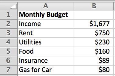Screen capture showing the Monthly Budget spreadsheet, indicating the following: A1 = Monthly Budget A2 = Income B2 = $1,677 A3 = Rent B3 = $750 A4 = Utilities B4 = $230 A5 = Food B5 = $160 A6 = Insurance B6 = $89 A7 = Gas for Car B7 = $80

Use this spreadsheet to answer Questions 6–8.

(6) What is in Cell B4?

(7) What does the number in Cell B4 represent in Lisa’s budget?

(i) The money she plans to spend on rent each month.

(ii) The money she plans to spend on utilities each month.

(iii) The money she plans to spend on food each month.

(iv) The money she plans to spend on insurance each month.

(v) The money she plans to spend on gas for her car each month.

Formulas and Spreadsheets

Formulas are algebraic expressions that show important and non-changing relationships. They can be used to perform calculations in spreadsheets. The formulas use the cell name as a variable that represents the value in that cell. For example, in the spreadsheet above, the formula “=B3+B4” would result in the calculation $750 + $230, and “$980” would be displayed. Spreadsheets are a valuable tool because once a formula is written, the result will change when the values change. So if Lisa’s rent increases, she can change the number in Cell B3 and the formula will calculate the new result(s) automatically.

(8) Lisa put the following formula in her spreadsheet:

=B2-B3-B4-B5-B6-B7

(a) Calculate the result of this formula.

(b) What does this value represent for Lisa?

(i) The amount of money she expects to lose each month.

(ii) The amount of money she expects to have left after paying bills each month.

(iii) The percentage of her income that she will be able to save each month.

(iv) The value has no meaning for Lisa.

(i) =B2-B3+B4+B5+B6+B7

(ii) =B2-(B3+B4+B5+B6+B7)

(iii) =(B3+B4+B5+B6+B7)-B2

(iv) =B3+B4+B5+B6+B7-B2

MAKING CONNECTIONS ACROSS THE COURSE

(9) Which of these expressions shows how to calculate 25% of 2,310? There may be more than one correct answer.

(i) 2,310 ÷ 4

(ii) 2,310 × 4

(iii) 2,310 ÷ 25

(iv) 2,310 × 25

(v) 2,310 × 0.25

(vi) 2,310 ÷ 0.25

(vii) $\dfrac{1}{4}$ × 2,310

(viii) $\dfrac{1}{4}$ ÷ 2,310

(ix) 0.25 × 2,310

(x) 0.25 ÷ 2,310

(10) Which expression is the same as 20% of a billion? There may be more than one correct answer.

(i) 0.2 × 1,000,000,000

(ii) 0.2 × 1,000,000

(iii) 10⁹ ÷ 5

(iv) 10⁹ ÷ 20

(v) 10⁶ ÷ 5

(vi) One-fifth of 1,000 million

(vii) 20,000,000

(viii) 20 ÷ 100 × 1,000,000,000

Scientific Notation

In Exercise 1.3, you saw that a large number can be written as a number times a power of 10 in many different ways. For example, the number 124,000 can be written as 1.24 × 10⁵ or 12.4 × 10⁴. These different forms are all equivalent.

Scientific notation is a very specific way to write a large number as a power of 10. The purpose of scientific notation is to make it easier for people to use and communicate with large numbers. It would be confusing if two people working together on one project wrote the same number in two different ways. To avoid this, people decided that numbers in scientific notation would always be written in the same way: a number between 1 and 10 times a power of 10.

From the previous example:

1.24 × 10⁵ is in scientific notation because 1.24 is a number between 1 and 10.
12.4 × 10⁴ is not in scientific notation because 12.4 is larger than 10.

(11) Write 16,900,000 in scientific notation.

(12) Write 4,275,000,000 in scientific notation.

Self-Regulating Your Learning: The Plan Phase

At the start of this module, the authors briefly described what it means to be a “self-regulated learner.” As you already learned, being a self-regulated learner involves going through three phases when you are working on a problem or an assignment. The phases are:

1. Plan

2. Work

3. Reflect

Let’s look at what you should be doing during the plan phase. As you might imagine, the planning phase involves thinking about all the things you need to do to successfully complete a problem or assignment before you begin working on it. As was said previously, researchers who study how people learn found that experts often spend a lot more time planning how they are going to finish a task than they spend actually doing the task.

The planning phase involves several important aspects. The following are some that will be explored in this course:

How much confidence you have that you can successfully complete the problem.
The amount of time and effort you think it will take to understand and work on the problem.
The strategies you might use to solve the problem.
The goals you have as you try to work on the problem.

The authors will now describe each aspect in a little more detail. You will also continue to revisit them throughout the rest of the course.

Confidence: People who study how we learn have found that our beliefs regarding our ability to do a given task, like work on a particular math problem, often predicts how well we will actually do. Here is one way to think about it: If you really believe you can succeed at a problem, you are more likely to keep trying and keep working on that problem even if you get stuck. Because you invest more effort, you are more likely to be successful. On the other hand, if you look at a problem and immediately think “I cannot do this,” then when you do get stuck or confused, you might be more likely to give up and not be successful. Researchers call your beliefs about your abilities your self-efficacy.

In this course, you will be asked to rate your self-efficacy on certain problems. If you rate yourself low, then you might want to allow more time to do that problem, plan to go get help, or try being more patient than you might normally be. Thinking about your confidence can help you plan your time and effort when you work on a problem or task.

Time and Effort: Obviously, some problems or assignments take more time than others. Some assignments require more effort than others. It can be frustrating to jump into an assignment thinking you can finish it easily or quickly only to discover it is harder or takes more time than you thought it would. You can avoid some or all of that frustration if you have a realistic idea of how hard the assignment will be. Also, having a good idea of how much time and effort will be needed helps you manage your time. For example, you might need to allocate time to discuss the assignment with your instructor, classmates, or tutors. For these reasons, approximating the time and effort needed before starting work on an assignment is a good planning tool.

Strategies: When you start working on a problem or assignment, you often have to try several different strategies before you find an approach that will help you complete it successfully. Sometimes, it is the first strategy you think of, but often it is not. If you think about possible strategies before you begin working, you immediately have another one to try if your first one does not work. Self-regulated learners think about many different possible strategies before trying to solve a problem.

Goals: Education researchers have shown that students who have learning goals are more likely to succeed than students who have what are called performance goals. If you have learning goals, you are trying to understand what you are learning and trying to make connections between ideas and concepts. If you have performance goals, you care most about finishing an assignment to get points or have it done; you are not focused on understanding the material. Self-regulated learners try to have learning goals more than performance goals. This helps them stay focused and motivated to learn when the problems are challenging. Good planning means making an effort to change your thinking so you have learning goals as often as possible.

In future collaborations and assignments, you will have opportunities to practice the planning ideas presented here. Before then, start incorporating the planning phase whenever you start an assignment. If you do, you will be better prepared and more likely to succeed.

General Rule	Example
\(\dfrac{a}{b} = a \times \dfrac{1}{b}\)	\(15 \div 5 = 15 \times \dfrac{1}{5}\)
\(a \div \dfrac{b}{c} = a \times \dfrac{c}{b}\)	\(10 \div \dfrac{3}{5} = 10 \times \dfrac{5}{3}\)

Search

Text Color

Text Size

Margin Size

Font Type

Multiplication	Division
85 × \(\dfrac{1}{5}\)	85 ÷ ___
1.23 × ___	1.23 ÷ 7
1.23 × ___	1.23 ÷ \(\dfrac{2}{3}\)