
2.7: Making Good Decisions with Good Statistics
- Page ID
- 148725

\( \newcommand{\vecs}[1]{\overset { \scriptstyle \rightharpoonup} {\mathbf{#1}} } \)
\( \newcommand{\vecd}[1]{\overset{-\!-\!\rightharpoonup}{\vphantom{a}\smash {#1}}} \)
\( \newcommand{\id}{\mathrm{id}}\) \( \newcommand{\Span}{\mathrm{span}}\)
( \newcommand{\kernel}{\mathrm{null}\,}\) \( \newcommand{\range}{\mathrm{range}\,}\)
\( \newcommand{\RealPart}{\mathrm{Re}}\) \( \newcommand{\ImaginaryPart}{\mathrm{Im}}\)
\( \newcommand{\Argument}{\mathrm{Arg}}\) \( \newcommand{\norm}[1]{\| #1 \|}\)
\( \newcommand{\inner}[2]{\langle #1, #2 \rangle}\)
\( \newcommand{\Span}{\mathrm{span}}\)
\( \newcommand{\id}{\mathrm{id}}\)
\( \newcommand{\Span}{\mathrm{span}}\)
\( \newcommand{\kernel}{\mathrm{null}\,}\)
\( \newcommand{\range}{\mathrm{range}\,}\)
\( \newcommand{\RealPart}{\mathrm{Re}}\)
\( \newcommand{\ImaginaryPart}{\mathrm{Im}}\)
\( \newcommand{\Argument}{\mathrm{Arg}}\)
\( \newcommand{\norm}[1]{\| #1 \|}\)
\( \newcommand{\inner}[2]{\langle #1, #2 \rangle}\)
\( \newcommand{\Span}{\mathrm{span}}\) \( \newcommand{\AA}{\unicode[.8,0]{x212B}}\)
\( \newcommand{\vectorA}[1]{\vec{#1}} % arrow\)
\( \newcommand{\vectorAt}[1]{\vec{\text{#1}}} % arrow\)
\( \newcommand{\vectorB}[1]{\overset { \scriptstyle \rightharpoonup} {\mathbf{#1}} } \)
\( \newcommand{\vectorC}[1]{\textbf{#1}} \)
\( \newcommand{\vectorD}[1]{\overrightarrow{#1}} \)
\( \newcommand{\vectorDt}[1]{\overrightarrow{\text{#1}}} \)
\( \newcommand{\vectE}[1]{\overset{-\!-\!\rightharpoonup}{\vphantom{a}\smash{\mathbf {#1}}}} \)
\( \newcommand{\vecs}[1]{\overset { \scriptstyle \rightharpoonup} {\mathbf{#1}} } \)
\( \newcommand{\vecd}[1]{\overset{-\!-\!\rightharpoonup}{\vphantom{a}\smash {#1}}} \)
\(\newcommand{\avec}{\mathbf a}\) \(\newcommand{\bvec}{\mathbf b}\) \(\newcommand{\cvec}{\mathbf c}\) \(\newcommand{\dvec}{\mathbf d}\) \(\newcommand{\dtil}{\widetilde{\mathbf d}}\) \(\newcommand{\evec}{\mathbf e}\) \(\newcommand{\fvec}{\mathbf f}\) \(\newcommand{\nvec}{\mathbf n}\) \(\newcommand{\pvec}{\mathbf p}\) \(\newcommand{\qvec}{\mathbf q}\) \(\newcommand{\svec}{\mathbf s}\) \(\newcommand{\tvec}{\mathbf t}\) \(\newcommand{\uvec}{\mathbf u}\) \(\newcommand{\vvec}{\mathbf v}\) \(\newcommand{\wvec}{\mathbf w}\) \(\newcommand{\xvec}{\mathbf x}\) \(\newcommand{\yvec}{\mathbf y}\) \(\newcommand{\zvec}{\mathbf z}\) \(\newcommand{\rvec}{\mathbf r}\) \(\newcommand{\mvec}{\mathbf m}\) \(\newcommand{\zerovec}{\mathbf 0}\) \(\newcommand{\onevec}{\mathbf 1}\) \(\newcommand{\real}{\mathbb R}\) \(\newcommand{\twovec}[2]{\left[\begin{array}{r}#1 \\ #2 \end{array}\right]}\) \(\newcommand{\ctwovec}[2]{\left[\begin{array}{c}#1 \\ #2 \end{array}\right]}\) \(\newcommand{\threevec}[3]{\left[\begin{array}{r}#1 \\ #2 \\ #3 \end{array}\right]}\) \(\newcommand{\cthreevec}[3]{\left[\begin{array}{c}#1 \\ #2 \\ #3 \end{array}\right]}\) \(\newcommand{\fourvec}[4]{\left[\begin{array}{r}#1 \\ #2 \\ #3 \\ #4 \end{array}\right]}\) \(\newcommand{\cfourvec}[4]{\left[\begin{array}{c}#1 \\ #2 \\ #3 \\ #4 \end{array}\right]}\) \(\newcommand{\fivevec}[5]{\left[\begin{array}{r}#1 \\ #2 \\ #3 \\ #4 \\ #5 \\ \end{array}\right]}\) \(\newcommand{\cfivevec}[5]{\left[\begin{array}{c}#1 \\ #2 \\ #3 \\ #4 \\ #5 \\ \end{array}\right]}\) \(\newcommand{\mattwo}[4]{\left[\begin{array}{rr}#1 \amp #2 \\ #3 \amp #4 \\ \end{array}\right]}\) \(\newcommand{\laspan}[1]{\text{Span}\{#1\}}\) \(\newcommand{\bcal}{\cal B}\) \(\newcommand{\ccal}{\cal C}\) \(\newcommand{\scal}{\cal S}\) \(\newcommand{\wcal}{\cal W}\) \(\newcommand{\ecal}{\cal E}\) \(\newcommand{\coords}[2]{\left\{#1\right\}_{#2}}\) \(\newcommand{\gray}[1]{\color{gray}{#1}}\) \(\newcommand{\lgray}[1]{\color{lightgray}{#1}}\) \(\newcommand{\rank}{\operatorname{rank}}\) \(\newcommand{\row}{\text{Row}}\) \(\newcommand{\col}{\text{Col}}\) \(\renewcommand{\row}{\text{Row}}\) \(\newcommand{\nul}{\text{Nul}}\) \(\newcommand{\var}{\text{Var}}\) \(\newcommand{\corr}{\text{corr}}\) \(\newcommand{\len}[1]{\left|#1\right|}\) \(\newcommand{\bbar}{\overline{\bvec}}\) \(\newcommand{\bhat}{\widehat{\bvec}}\) \(\newcommand{\bperp}{\bvec^\perp}\) \(\newcommand{\xhat}{\widehat{\xvec}}\) \(\newcommand{\vhat}{\widehat{\vvec}}\) \(\newcommand{\uhat}{\widehat{\uvec}}\) \(\newcommand{\what}{\widehat{\wvec}}\) \(\newcommand{\Sighat}{\widehat{\Sigma}}\) \(\newcommand{\lt}{<}\) \(\newcommand{\gt}{>}\) \(\newcommand{\amp}{&}\) \(\definecolor{fillinmathshade}{gray}{0.9}\)INTRODUCTION
Imagine you have been offered a job at one of the following companies. Which one would you pick based only on the two salary descriptions below, and why? Discuss in your group and be prepared to support your reasoning.
- Company A: average salary $105,000 per year
- Company B: median salary $80,000 per year
|
Position |
Company A |
Company B |
|
Secretary |
$45,000 |
$52,000 |
|
Sales representative |
$47,000 |
$70,000 |
|
Sales representative |
$52,000 |
$75,000 |
|
Security officer |
$53,000 |
$80,000 |
|
Security officer |
$53,000 |
$81,000 |
|
Warehouse manager |
$55,000 |
$86,000 |
|
CEO |
$240,000 |
$286,000 |
|
Mean (average) salary $105,000 |
Median salary $80,000 |
SPECIFIC OBJECTIVES
By the end of this collaboration, you should understand that
- each statistic—the mean, median, and mode—is a different summary of numerical data.
- conclusions derived from statistical summaries are subject to error.
- measures of central tendency can be used to make decisions.
By the end of this collaboration, you should be able to
- make good decisions using information about data.
- interpret the mean, median, or mode in terms of the context of the problem.
- match data sets with appropriate statistics.
PROBLEM SITUATION 1: MAKING SENSE OF MEASURES OF CENTRAL TENDENCY
Examine the following three advertisements.
Employment Opportunities
|
Sales Positions Available! We have immediate need for five enthusiastic self-starters who love the outdoors and who love people. Our salespeople make an average of $1,000 per week. Come join the winning team. Call 555-0100 now! |
Are you above average? Our company is hiring one person this month—will you be that person? We pay the top percentage commission and supply you leads. Half of our sales force makes over $3,000 per month. Join the Call 555-0127 now! We are! |
NEED A NEW CHALLENGE? Join a super sales force and make as much as you want. Five of our nine salespeople closed FOUR homes last month. Their average commission was $1,500 on each sale. Do the math—this is the job for you. Making dreams real— call 555-0199 |
(1) (a) Identify any measures of central tendency and how they are used in each advertisement.
(b) For each advertisement, create a set of data that fits the description. Note that this exercise is similar to the one in Collaboration 2.6 where you made a list of credit card debts for the five college students.
(2) In which job would you expect to earn the most money? Discuss in your group.
PROBLEM SITUATION 2: UNDERSTANDING TRENDS IN DATA
The median and average sales price of new homes sold in the United States from 1963–2022 are shown in the following graph.23
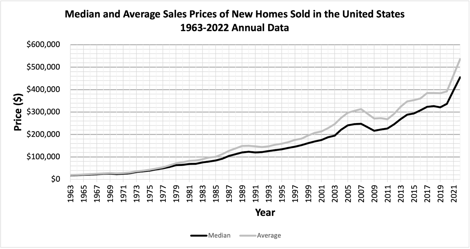
(3) Examine the graph and write at least three statements about the data. Recall the Writing Principle: Use specific and complete information.
(4) Table 1 gives a sample data set of home prices that matches the data shown in Graph 1 for the year 1977. And five possible data sets for the year 2019 are given in Table 2. Use your knowledge of mean and median to answer the following questions without calculating the mean of the data sets. There may be more than one correct answer to any of the questions.
|
Table 1: Sales Prices of a Sample of New Homes
|
Table 2: Possible Data Sets for 2019
|
(a) Which of the data sets could represent the data in the graph?
(b) Which of the data sets would likely have a mean that is less than the median?
(c) Which of the data sets would likely have a mean and median that are close together?
MAKING CONNECTIONS
Record the important mathematical ideas from the discussion.
__________________________________