
3.6.1: Preparation 3.6
- Page ID
- 148752

\( \newcommand{\vecs}[1]{\overset { \scriptstyle \rightharpoonup} {\mathbf{#1}} } \)
\( \newcommand{\vecd}[1]{\overset{-\!-\!\rightharpoonup}{\vphantom{a}\smash {#1}}} \)
\( \newcommand{\id}{\mathrm{id}}\) \( \newcommand{\Span}{\mathrm{span}}\)
( \newcommand{\kernel}{\mathrm{null}\,}\) \( \newcommand{\range}{\mathrm{range}\,}\)
\( \newcommand{\RealPart}{\mathrm{Re}}\) \( \newcommand{\ImaginaryPart}{\mathrm{Im}}\)
\( \newcommand{\Argument}{\mathrm{Arg}}\) \( \newcommand{\norm}[1]{\| #1 \|}\)
\( \newcommand{\inner}[2]{\langle #1, #2 \rangle}\)
\( \newcommand{\Span}{\mathrm{span}}\)
\( \newcommand{\id}{\mathrm{id}}\)
\( \newcommand{\Span}{\mathrm{span}}\)
\( \newcommand{\kernel}{\mathrm{null}\,}\)
\( \newcommand{\range}{\mathrm{range}\,}\)
\( \newcommand{\RealPart}{\mathrm{Re}}\)
\( \newcommand{\ImaginaryPart}{\mathrm{Im}}\)
\( \newcommand{\Argument}{\mathrm{Arg}}\)
\( \newcommand{\norm}[1]{\| #1 \|}\)
\( \newcommand{\inner}[2]{\langle #1, #2 \rangle}\)
\( \newcommand{\Span}{\mathrm{span}}\) \( \newcommand{\AA}{\unicode[.8,0]{x212B}}\)
\( \newcommand{\vectorA}[1]{\vec{#1}} % arrow\)
\( \newcommand{\vectorAt}[1]{\vec{\text{#1}}} % arrow\)
\( \newcommand{\vectorB}[1]{\overset { \scriptstyle \rightharpoonup} {\mathbf{#1}} } \)
\( \newcommand{\vectorC}[1]{\textbf{#1}} \)
\( \newcommand{\vectorD}[1]{\overrightarrow{#1}} \)
\( \newcommand{\vectorDt}[1]{\overrightarrow{\text{#1}}} \)
\( \newcommand{\vectE}[1]{\overset{-\!-\!\rightharpoonup}{\vphantom{a}\smash{\mathbf {#1}}}} \)
\( \newcommand{\vecs}[1]{\overset { \scriptstyle \rightharpoonup} {\mathbf{#1}} } \)
\( \newcommand{\vecd}[1]{\overset{-\!-\!\rightharpoonup}{\vphantom{a}\smash {#1}}} \)
\(\newcommand{\avec}{\mathbf a}\) \(\newcommand{\bvec}{\mathbf b}\) \(\newcommand{\cvec}{\mathbf c}\) \(\newcommand{\dvec}{\mathbf d}\) \(\newcommand{\dtil}{\widetilde{\mathbf d}}\) \(\newcommand{\evec}{\mathbf e}\) \(\newcommand{\fvec}{\mathbf f}\) \(\newcommand{\nvec}{\mathbf n}\) \(\newcommand{\pvec}{\mathbf p}\) \(\newcommand{\qvec}{\mathbf q}\) \(\newcommand{\svec}{\mathbf s}\) \(\newcommand{\tvec}{\mathbf t}\) \(\newcommand{\uvec}{\mathbf u}\) \(\newcommand{\vvec}{\mathbf v}\) \(\newcommand{\wvec}{\mathbf w}\) \(\newcommand{\xvec}{\mathbf x}\) \(\newcommand{\yvec}{\mathbf y}\) \(\newcommand{\zvec}{\mathbf z}\) \(\newcommand{\rvec}{\mathbf r}\) \(\newcommand{\mvec}{\mathbf m}\) \(\newcommand{\zerovec}{\mathbf 0}\) \(\newcommand{\onevec}{\mathbf 1}\) \(\newcommand{\real}{\mathbb R}\) \(\newcommand{\twovec}[2]{\left[\begin{array}{r}#1 \\ #2 \end{array}\right]}\) \(\newcommand{\ctwovec}[2]{\left[\begin{array}{c}#1 \\ #2 \end{array}\right]}\) \(\newcommand{\threevec}[3]{\left[\begin{array}{r}#1 \\ #2 \\ #3 \end{array}\right]}\) \(\newcommand{\cthreevec}[3]{\left[\begin{array}{c}#1 \\ #2 \\ #3 \end{array}\right]}\) \(\newcommand{\fourvec}[4]{\left[\begin{array}{r}#1 \\ #2 \\ #3 \\ #4 \end{array}\right]}\) \(\newcommand{\cfourvec}[4]{\left[\begin{array}{c}#1 \\ #2 \\ #3 \\ #4 \end{array}\right]}\) \(\newcommand{\fivevec}[5]{\left[\begin{array}{r}#1 \\ #2 \\ #3 \\ #4 \\ #5 \\ \end{array}\right]}\) \(\newcommand{\cfivevec}[5]{\left[\begin{array}{c}#1 \\ #2 \\ #3 \\ #4 \\ #5 \\ \end{array}\right]}\) \(\newcommand{\mattwo}[4]{\left[\begin{array}{rr}#1 \amp #2 \\ #3 \amp #4 \\ \end{array}\right]}\) \(\newcommand{\laspan}[1]{\text{Span}\{#1\}}\) \(\newcommand{\bcal}{\cal B}\) \(\newcommand{\ccal}{\cal C}\) \(\newcommand{\scal}{\cal S}\) \(\newcommand{\wcal}{\cal W}\) \(\newcommand{\ecal}{\cal E}\) \(\newcommand{\coords}[2]{\left\{#1\right\}_{#2}}\) \(\newcommand{\gray}[1]{\color{gray}{#1}}\) \(\newcommand{\lgray}[1]{\color{lightgray}{#1}}\) \(\newcommand{\rank}{\operatorname{rank}}\) \(\newcommand{\row}{\text{Row}}\) \(\newcommand{\col}{\text{Col}}\) \(\renewcommand{\row}{\text{Row}}\) \(\newcommand{\nul}{\text{Nul}}\) \(\newcommand{\var}{\text{Var}}\) \(\newcommand{\corr}{\text{corr}}\) \(\newcommand{\len}[1]{\left|#1\right|}\) \(\newcommand{\bbar}{\overline{\bvec}}\) \(\newcommand{\bhat}{\widehat{\bvec}}\) \(\newcommand{\bperp}{\bvec^\perp}\) \(\newcommand{\xhat}{\widehat{\xvec}}\) \(\newcommand{\vhat}{\widehat{\vvec}}\) \(\newcommand{\uhat}{\widehat{\uvec}}\) \(\newcommand{\what}{\widehat{\wvec}}\) \(\newcommand{\Sighat}{\widehat{\Sigma}}\) \(\newcommand{\lt}{<}\) \(\newcommand{\gt}{>}\) \(\newcommand{\amp}{&}\) \(\definecolor{fillinmathshade}{gray}{0.9}\)This preparation will help you prepare for both Collaboration 3.6 and Module 4. In the next module, you will make graphs on a coordinate plane like the one shown below. Over the next few assignments, you will learn about using a coordinate plane and practice how to graph points. This material is spread over several Exercises to give you time to be fully prepared for Module 4.
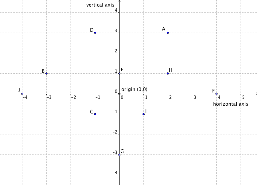
You will begin with some vocabulary. A coordinate plane has two axes that measure distance in two dimensions. The horizontal axis goes from left to right. In previous classes, you may have called this the x-axis. The vertical axis goes up and down. This is sometimes called the y-axis. The axes are two number lines that create a grid on the coordinate plane. (Note: Axis is singular and axes is plural.)
The point at which the two axes intersect or cross is called the origin. This point represents 0 for both axes. To the left of this point, the horizontal axis is negative; to the right it is positive. Below the origin, the vertical axis is negative; above the origin it is positive. You can see this in the numbers along each axis above. These numbers are called the scale.
Each location or point on the coordinate plane is defined by an ordered pair. You can think of this as the address of a point. An ordered pair must contain two numbers. Ordered pairs are written in a set of parentheses ( ) with a comma separating the numbers, such as (2, 4). The first number is the distance and direction going left or right from the origin and the second number is the distance and direction going up or down. The ordered pair for the origin is (0, 0).
Follow these steps to find the point represented by the ordered pair (2, 3):
- First, think about the “address” of the point. If this were a street address, the ordered pair tells you to walk 2 blocks horizontally in the positive direction (right) and then walk 3 units vertically in the positive direction (up).
- Start at the origin. Go 2 units to the right because this is the positive side of the horizontal axis.
- Go 3 units up.
Point A on the graph above is the point (2, 3). A few other examples from the graph are given below:
Point B: (–3, 1)
Point E: (0, 1)
Point F: (4, 0)
(1) Write the ordered pairs for the following points on the graph.
Point C:
Point D:
Point G:
Point H:
Point I:
Point J:
Statement of Equality
Remember that an equation is a statement of equality, meaning that it tells you that two expressions are equal to each other. An equation can be as simple as 3 = 3 or it can have complicated expressions with multiple terms on one or both sides of the equal sign. One of the most important things to remember is that if the value of one side of an equation is changed, then it is no longer an equation because the two sides are no longer equal. If you need to change the value of one side and you want to keep the equation true, you must change the value of the other side in the same way.
(2) Each of the following examples starts with the equation 3 = 3. Then a new operation is performed to one or both expressions. The new operations are shown in bold. If the new operations maintain the statement of equality, put an equal sign (=) in the blank. If the new operations do not maintain the statement of equality, put a not-equal sign (≠) in the blank.
|
(a) 3 = 3 3 + 2 ____ 3 + 2 |
(b) 3 = 3 2 + 3 ____ 3 + 2 |
|
(c) 3 = 3 5 + 3 ____ 4 + 3 |
(d) 3 = 3 0.5 × 3 ____ 3 × 1/2 |
|
(e) 3 = 3 3 ÷ 2 ____ 3 × 2 |
(f) 3 = 3 6 – 3 ____ 3 – 6 |
It is important to note that you are talking about changes to the value of an expression. Remember that there are multiple ways to write expressions without changing their value. For example, if you change 1/2 to 2/4, you have not changed the value because you have changed the fraction into an equivalent form.
(3) The following examples start with the equation 2x + 3x + 1 = 11. Then an operation, shown in bold, is performed on one or both expressions. If the new expressions maintain the statement of equality, put an equal sign (=) in the blank. If the new operations do not maintain the statement of equality, put a not-equal sign (≠) in the blank.
|
(a) 2x + 3x + 1 = 11 5x + 1 ____ 11 |
(b) 2x + 3x + 1 = 11 x + x + 3x + 1 ____ 11 |
|
(c) 2x + 3x + 1 = 11 6x ____ 11 |
(d) 2x + 3x + 1 = 11 2x + 3x + 1 – 1 ____ 11 |
|
(e) 2x + 3x + 1 = 11 2x + 3x + 1 – 1 ____ 11 – 1 |
The equation in Question 3 contains a variable that represents an unknown value. In an equation like this, there may be one or more values that can be substituted in for the variable to make a true equation. This is called a solution to an equation.
(4) Determine if each of the following is a solution to the equation 2x + 3x + 1 = 11. Write “solution” or “not a solution” for each.
(a) x = –2
(b) x = 2
(c) x = 0
After Preparation 3.6 (survey)
You should be able to do the following things for the next collaboration. Rate how confident you are on a scale of 1–5 (1 = not confident and 5 = very confident).
Before beginning Collaboration 3.6, you should understand the concepts and demonstrate the skills listed below.
|
Skill or Concept: I can … |
Rating from 1 to 5 |
|
understand the use of variables in mathematical equations. |
|
|
substitute a value for a variable in a mathematical equation and simplify the equation. |
|
|
understand that an equation is a statement of equality. |