
4.1.1: Preparation 4.1
- Page ID
- 148763

\( \newcommand{\vecs}[1]{\overset { \scriptstyle \rightharpoonup} {\mathbf{#1}} } \)
\( \newcommand{\vecd}[1]{\overset{-\!-\!\rightharpoonup}{\vphantom{a}\smash {#1}}} \)
\( \newcommand{\id}{\mathrm{id}}\) \( \newcommand{\Span}{\mathrm{span}}\)
( \newcommand{\kernel}{\mathrm{null}\,}\) \( \newcommand{\range}{\mathrm{range}\,}\)
\( \newcommand{\RealPart}{\mathrm{Re}}\) \( \newcommand{\ImaginaryPart}{\mathrm{Im}}\)
\( \newcommand{\Argument}{\mathrm{Arg}}\) \( \newcommand{\norm}[1]{\| #1 \|}\)
\( \newcommand{\inner}[2]{\langle #1, #2 \rangle}\)
\( \newcommand{\Span}{\mathrm{span}}\)
\( \newcommand{\id}{\mathrm{id}}\)
\( \newcommand{\Span}{\mathrm{span}}\)
\( \newcommand{\kernel}{\mathrm{null}\,}\)
\( \newcommand{\range}{\mathrm{range}\,}\)
\( \newcommand{\RealPart}{\mathrm{Re}}\)
\( \newcommand{\ImaginaryPart}{\mathrm{Im}}\)
\( \newcommand{\Argument}{\mathrm{Arg}}\)
\( \newcommand{\norm}[1]{\| #1 \|}\)
\( \newcommand{\inner}[2]{\langle #1, #2 \rangle}\)
\( \newcommand{\Span}{\mathrm{span}}\) \( \newcommand{\AA}{\unicode[.8,0]{x212B}}\)
\( \newcommand{\vectorA}[1]{\vec{#1}} % arrow\)
\( \newcommand{\vectorAt}[1]{\vec{\text{#1}}} % arrow\)
\( \newcommand{\vectorB}[1]{\overset { \scriptstyle \rightharpoonup} {\mathbf{#1}} } \)
\( \newcommand{\vectorC}[1]{\textbf{#1}} \)
\( \newcommand{\vectorD}[1]{\overrightarrow{#1}} \)
\( \newcommand{\vectorDt}[1]{\overrightarrow{\text{#1}}} \)
\( \newcommand{\vectE}[1]{\overset{-\!-\!\rightharpoonup}{\vphantom{a}\smash{\mathbf {#1}}}} \)
\( \newcommand{\vecs}[1]{\overset { \scriptstyle \rightharpoonup} {\mathbf{#1}} } \)
\( \newcommand{\vecd}[1]{\overset{-\!-\!\rightharpoonup}{\vphantom{a}\smash {#1}}} \)
\(\newcommand{\avec}{\mathbf a}\) \(\newcommand{\bvec}{\mathbf b}\) \(\newcommand{\cvec}{\mathbf c}\) \(\newcommand{\dvec}{\mathbf d}\) \(\newcommand{\dtil}{\widetilde{\mathbf d}}\) \(\newcommand{\evec}{\mathbf e}\) \(\newcommand{\fvec}{\mathbf f}\) \(\newcommand{\nvec}{\mathbf n}\) \(\newcommand{\pvec}{\mathbf p}\) \(\newcommand{\qvec}{\mathbf q}\) \(\newcommand{\svec}{\mathbf s}\) \(\newcommand{\tvec}{\mathbf t}\) \(\newcommand{\uvec}{\mathbf u}\) \(\newcommand{\vvec}{\mathbf v}\) \(\newcommand{\wvec}{\mathbf w}\) \(\newcommand{\xvec}{\mathbf x}\) \(\newcommand{\yvec}{\mathbf y}\) \(\newcommand{\zvec}{\mathbf z}\) \(\newcommand{\rvec}{\mathbf r}\) \(\newcommand{\mvec}{\mathbf m}\) \(\newcommand{\zerovec}{\mathbf 0}\) \(\newcommand{\onevec}{\mathbf 1}\) \(\newcommand{\real}{\mathbb R}\) \(\newcommand{\twovec}[2]{\left[\begin{array}{r}#1 \\ #2 \end{array}\right]}\) \(\newcommand{\ctwovec}[2]{\left[\begin{array}{c}#1 \\ #2 \end{array}\right]}\) \(\newcommand{\threevec}[3]{\left[\begin{array}{r}#1 \\ #2 \\ #3 \end{array}\right]}\) \(\newcommand{\cthreevec}[3]{\left[\begin{array}{c}#1 \\ #2 \\ #3 \end{array}\right]}\) \(\newcommand{\fourvec}[4]{\left[\begin{array}{r}#1 \\ #2 \\ #3 \\ #4 \end{array}\right]}\) \(\newcommand{\cfourvec}[4]{\left[\begin{array}{c}#1 \\ #2 \\ #3 \\ #4 \end{array}\right]}\) \(\newcommand{\fivevec}[5]{\left[\begin{array}{r}#1 \\ #2 \\ #3 \\ #4 \\ #5 \\ \end{array}\right]}\) \(\newcommand{\cfivevec}[5]{\left[\begin{array}{c}#1 \\ #2 \\ #3 \\ #4 \\ #5 \\ \end{array}\right]}\) \(\newcommand{\mattwo}[4]{\left[\begin{array}{rr}#1 \amp #2 \\ #3 \amp #4 \\ \end{array}\right]}\) \(\newcommand{\laspan}[1]{\text{Span}\{#1\}}\) \(\newcommand{\bcal}{\cal B}\) \(\newcommand{\ccal}{\cal C}\) \(\newcommand{\scal}{\cal S}\) \(\newcommand{\wcal}{\cal W}\) \(\newcommand{\ecal}{\cal E}\) \(\newcommand{\coords}[2]{\left\{#1\right\}_{#2}}\) \(\newcommand{\gray}[1]{\color{gray}{#1}}\) \(\newcommand{\lgray}[1]{\color{lightgray}{#1}}\) \(\newcommand{\rank}{\operatorname{rank}}\) \(\newcommand{\row}{\text{Row}}\) \(\newcommand{\col}{\text{Col}}\) \(\renewcommand{\row}{\text{Row}}\) \(\newcommand{\nul}{\text{Nul}}\) \(\newcommand{\var}{\text{Var}}\) \(\newcommand{\corr}{\text{corr}}\) \(\newcommand{\len}[1]{\left|#1\right|}\) \(\newcommand{\bbar}{\overline{\bvec}}\) \(\newcommand{\bhat}{\widehat{\bvec}}\) \(\newcommand{\bperp}{\bvec^\perp}\) \(\newcommand{\xhat}{\widehat{\xvec}}\) \(\newcommand{\vhat}{\widehat{\vvec}}\) \(\newcommand{\uhat}{\widehat{\uvec}}\) \(\newcommand{\what}{\widehat{\wvec}}\) \(\newcommand{\Sighat}{\widehat{\Sigma}}\) \(\newcommand{\lt}{<}\) \(\newcommand{\gt}{>}\) \(\newcommand{\amp}{&}\) \(\definecolor{fillinmathshade}{gray}{0.9}\)Model or Equation
In Collaboration 3.2, your class wrote a mathematical equation for the relationship. An equation is useful because it can be used to calculate the cost values. As you saw with the formula for braking distance in Collaboration 3.4, equations are also useful for communicating complex relationships. In writing equations, it is always important to define what the variables represent, including units. For example, in Collaboration 3.2, the variables were defined as shown below. Note that each definition includes what the variable represents, such as cost of Jenna’s car, and the units in which this quantity is measured, such as $/mile.
J = Cost of Jenna’s car in $/mile
g = Price of gas ($/gal)
These variables were used in the mathematical equation, \(J = \dfrac{g}{18} + 0.0626\).
Table
Another way that you could have represented this relationship between the price of gas and the cost of driving the car is in a table that shows values of g and D as ordered pairs. An ordered pair is two values that are matched together in a given relationship. You used this representation in Collaboration 3.4 when you explored how one variable affected another. Tables are helpful for recognizing patterns and general relationships or for giving information about specific values. A table should always have labels for each column. The labels should include units when appropriate.
|
Price of Gas ($/gal) |
Cost of Driving Jenna’s Car ($/mile) |
|
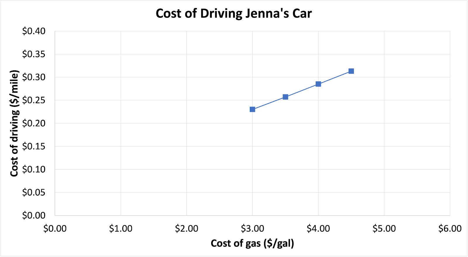
3.00 |
0.23 |
|
3.50 |
0.26 |
|
4.00 |
0.28 |
|
4.50 |
0.31 |
Graph
A graph provides a visual representation of the situation. It helps you see how the variables are related to each other, and it helps you to make predictions about future values or values in between those in your table. The horizontal and vertical axis of the graph should be labeled, including units.
Verbal Description
A verbal description explains the relationship in words. As discussed in Collaboration 3.4, some relationships are difficult to put into words, while in other cases a verbal description can help you make sense of what the relationship means in the context. The verbal description for Jenna’s car is too complex to discuss here. You will see examples of verbal descriptions in the next lesson.
Summary
Throughout this course, you have learned that having the skill to move between different forms and tools is important in problem solving. Alternating among the four representations of mathematical relationships is another example of this. In some cases, you may struggle with writing an equation, but find it helpful to start with a table . You might want a graph for a visual representation, but also need to express a relationship in words. It is important that you can translate one form into another and also that you can choose which form is most useful in a specific situation.
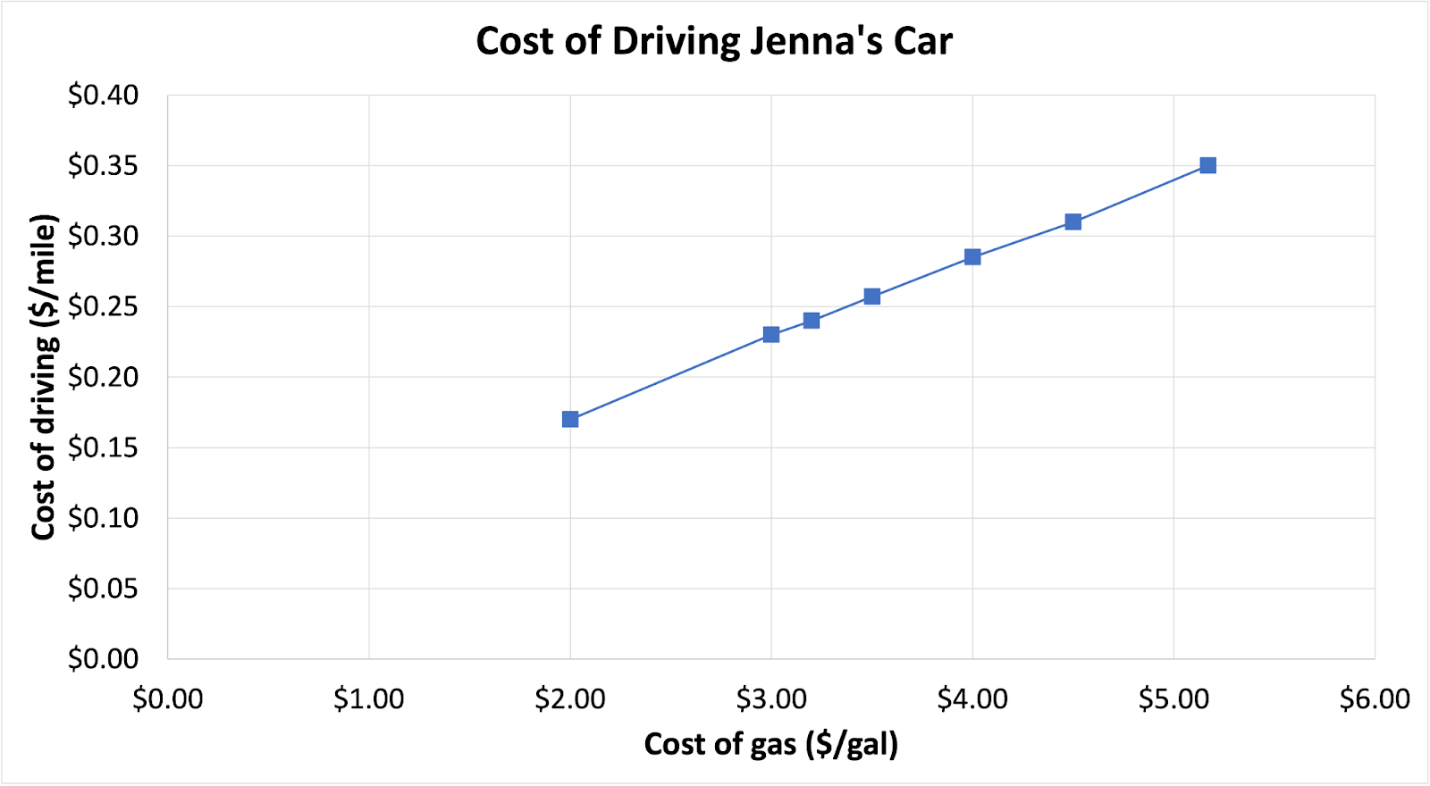
You will practice these skills with the following questions using the above situation of finding the cost of driving Jenna’s car.
(1) Complete the three missing entries in the table:
|
Price of Gas ($/gal) |
Cost of Driving Jenna’s Car ($/mile) |
|
2.00 |
|
|
3.00 |
0.23 |
|
3.20 |
|
|
3.50 |
0.26 |
|
4.00 |
0.28 |
|
4.50 |
0.31 |
|
0.35 |
(2) Use the graph to estimate the cost of driving if gas is $2.50/gallon.
After Preparation 4.1 (survey)
You should be able to do the following things for the next collaboration. Rate how confident you are on a scale of 1–5 (1 = not confident and 5 = very confident).
Before beginning Collaboration 4.1, you should understand the concepts and demonstrate the skills listed below:
|
Skill or Concept: I can … |
Rating from 1 to 5 |
|
understand the basic meaning and use of variables. |
|
|
solve for an unknown variable in a one-variable equation. |
|
|
graph points on a coordinate plane. |