4.3: That Is Close Enough

Last updated
Save as PDF

Page ID: 148768

$ \newcommand{\vecs}[1]{\overset { \scriptstyle \rightharpoonup} {\mathbf{#1}} } $

$ \newcommand{\vecd}[1]{\overset{-\!-\!\rightharpoonup}{\vphantom{a}\smash {#1}}} $

$ \newcommand{\id}{\mathrm{id}}$ $ \newcommand{\Span}{\mathrm{span}}$

( \newcommand{\kernel}{\mathrm{null}\,}\) $ \newcommand{\range}{\mathrm{range}\,}$

$ \newcommand{\RealPart}{\mathrm{Re}}$ $ \newcommand{\ImaginaryPart}{\mathrm{Im}}$

$ \newcommand{\Argument}{\mathrm{Arg}}$ $ \newcommand{\norm}[1]{\| #1 \|}$

$ \newcommand{\inner}[2]{\langle #1, #2 \rangle}$

$ \newcommand{\Span}{\mathrm{span}}$

$ \newcommand{\id}{\mathrm{id}}$

$ \newcommand{\Span}{\mathrm{span}}$

$ \newcommand{\kernel}{\mathrm{null}\,}$

$ \newcommand{\range}{\mathrm{range}\,}$

$ \newcommand{\RealPart}{\mathrm{Re}}$

$ \newcommand{\ImaginaryPart}{\mathrm{Im}}$

$ \newcommand{\Argument}{\mathrm{Arg}}$

$ \newcommand{\norm}[1]{\| #1 \|}$

$ \newcommand{\inner}[2]{\langle #1, #2 \rangle}$

$ \newcommand{\Span}{\mathrm{span}}$ $ \newcommand{\AA}{\unicode[.8,0]{x212B}}$

$ \newcommand{\vectorA}[1]{\vec{#1}} % arrow$

$ \newcommand{\vectorAt}[1]{\vec{\text{#1}}} % arrow$

$ \newcommand{\vectorB}[1]{\overset { \scriptstyle \rightharpoonup} {\mathbf{#1}} } $

$ \newcommand{\vectorC}[1]{\textbf{#1}} $

$ \newcommand{\vectorD}[1]{\overrightarrow{#1}} $

$ \newcommand{\vectorDt}[1]{\overrightarrow{\text{#1}}} $

$ \newcommand{\vectE}[1]{\overset{-\!-\!\rightharpoonup}{\vphantom{a}\smash{\mathbf {#1}}}} $

$ \newcommand{\vecs}[1]{\overset { \scriptstyle \rightharpoonup} {\mathbf{#1}} } $

$ \newcommand{\vecd}[1]{\overset{-\!-\!\rightharpoonup}{\vphantom{a}\smash {#1}}} $

$\newcommand{\avec}{\mathbf a}$ $\newcommand{\bvec}{\mathbf b}$ $\newcommand{\cvec}{\mathbf c}$ $\newcommand{\dvec}{\mathbf d}$ $\newcommand{\dtil}{\widetilde{\mathbf d}}$ $\newcommand{\evec}{\mathbf e}$ $\newcommand{\fvec}{\mathbf f}$ $\newcommand{\nvec}{\mathbf n}$ $\newcommand{\pvec}{\mathbf p}$ $\newcommand{\qvec}{\mathbf q}$ $\newcommand{\svec}{\mathbf s}$ $\newcommand{\tvec}{\mathbf t}$ $\newcommand{\uvec}{\mathbf u}$ $\newcommand{\vvec}{\mathbf v}$ $\newcommand{\wvec}{\mathbf w}$ $\newcommand{\xvec}{\mathbf x}$ $\newcommand{\yvec}{\mathbf y}$ $\newcommand{\zvec}{\mathbf z}$ $\newcommand{\rvec}{\mathbf r}$ $\newcommand{\mvec}{\mathbf m}$ $\newcommand{\zerovec}{\mathbf 0}$ $\newcommand{\onevec}{\mathbf 1}$ $\newcommand{\real}{\mathbb R}$ $\newcommand{\twovec}[2]{\left[\begin{array}{r}#1 \\ #2 \end{array}\right]}$ $\newcommand{\ctwovec}[2]{\left[\begin{array}{c}#1 \\ #2 \end{array}\right]}$ $\newcommand{\threevec}[3]{\left[\begin{array}{r}#1 \\ #2 \\ #3 \end{array}\right]}$ $\newcommand{\cthreevec}[3]{\left[\begin{array}{c}#1 \\ #2 \\ #3 \end{array}\right]}$ $\newcommand{\fourvec}[4]{\left[\begin{array}{r}#1 \\ #2 \\ #3 \\ #4 \end{array}\right]}$ $\newcommand{\cfourvec}[4]{\left[\begin{array}{c}#1 \\ #2 \\ #3 \\ #4 \end{array}\right]}$ $\newcommand{\fivevec}[5]{\left[\begin{array}{r}#1 \\ #2 \\ #3 \\ #4 \\ #5 \\ \end{array}\right]}$ $\newcommand{\cfivevec}[5]{\left[\begin{array}{c}#1 \\ #2 \\ #3 \\ #4 \\ #5 \\ \end{array}\right]}$ $\newcommand{\mattwo}[4]{\left[\begin{array}{rr}#1 \amp #2 \\ #3 \amp #4 \\ \end{array}\right]}$ $\newcommand{\laspan}[1]{\text{Span}\{#1\}}$ $\newcommand{\bcal}{\cal B}$ $\newcommand{\ccal}{\cal C}$ $\newcommand{\scal}{\cal S}$ $\newcommand{\wcal}{\cal W}$ $\newcommand{\ecal}{\cal E}$ $\newcommand{\coords}[2]{\left\{#1\right\}_{#2}}$ $\newcommand{\gray}[1]{\color{gray}{#1}}$ $\newcommand{\lgray}[1]{\color{lightgray}{#1}}$ $\newcommand{\rank}{\operatorname{rank}}$ $\newcommand{\row}{\text{Row}}$ $\newcommand{\col}{\text{Col}}$ $\renewcommand{\row}{\text{Row}}$ $\newcommand{\nul}{\text{Nul}}$ $\newcommand{\var}{\text{Var}}$ $\newcommand{\corr}{\text{corr}}$ $\newcommand{\len}[1]{\left|#1\right|}$ $\newcommand{\bbar}{\overline{\bvec}}$ $\newcommand{\bhat}{\widehat{\bvec}}$ $\newcommand{\bperp}{\bvec^\perp}$ $\newcommand{\xhat}{\widehat{\xvec}}$ $\newcommand{\vhat}{\widehat{\vvec}}$ $\newcommand{\uhat}{\widehat{\uvec}}$ $\newcommand{\what}{\widehat{\wvec}}$ $\newcommand{\Sighat}{\widehat{\Sigma}}$ $\newcommand{\lt}{<}$ $\newcommand{\gt}{>}$ $\newcommand{\amp}{&}$ $\definecolor{fillinmathshade}{gray}{0.9}$

INTRODUCTION

Recall the information in Preparation 4.3 about Social Security Reform. Refresh your memory by reading the information below and note any questions you have before discussing the prompts below in your group.

There is concern about the Social Security program because it is projected to eventually run out of money. Based on the current program, the Social Security program is projected to be able to pay all benefits through the year 2033. After that, it will only take in enough money to pay three-fourths of benefits. There is broad agreement that the program should be reformed now to avoid this future budget problem, but there is not an agreement about how that should be done.

The following are possible solutions that have been proposed:

Increase the tax rate for paying into Social Security.
Increase the limit on wages so that people pay Social Security on wages above $160,200.
Decrease future benefits.
Increase the retirement age.
Change the program into a system of private retirement accounts in which individuals invest their own money.

Projections about Social Security are based on many variables. One of these is life expectancy. Life expectancy is a prediction about how long people live on average. It is important to understand that this is a mean. When you studied mean in Module 2, you learned that a data set can have values far above or below the mean. If a large group of people has a life expectancy of 63 years, some people will die very young, even as infants, and some will live to be over 100.

This might lead you to ask if using a mean to measure life expectancy is very accurate. In Collaboration 2.7, you saw data sets with home prices in which the mean was not a good representation of the data because there were a few very high home prices that made the mean much higher than most of the data. Prices of luxury homes can be 10 or 20 times higher than the price of “average” homes. This makes the mean a poor representation of the data. The range of life expectancy is different because it has more defined limits. As of 2023, the person known to have lived the longest was Jeanne Calment, who died at the age of 122 in 1997. This is an extremely high age, but it is rare and represents the maximum possible age known. So, although it is twice an average age in the range of 60–70 years, it would not have much impact on the mean. This indicates that the mean is a fairly accurate way to summarize the data. This is useful when making projections about a large population. This is why life expectancy statistics are used for projecting costs for Social Security. But you should remember that these types of statistics are not always good predictors for individuals.

Discuss in your group any questions you have.
Do you think the Social Security retirement age should be raised or whether other methods should be used to reform the system? Justify your reasons.
Do you think life expectancy is different for certain populations in the United States?

SPECIFIC OBJECTIVES

By the end of this collaboration, you should understand that

linear equations can approximate nearly linear data.

By the end of this collaboration, you should be able to

find the equation of a line that estimates nearly linear data by calculating the rate of change and estimating the vertical intercept of the line.
use approximate linear models to interpolate and extrapolate.

PROBLEM SITUATION: LIFE EXPECTANCY AND SOCIAL SECURITY

As you read in Preparation 4.3, one proposal to reform Social Security is to increase the retirement age. This, however, raises concerns about fairness. No matter what the retirement age is, some people will pay into Social Security but die before retirement and never receive a benefit. This happens to more people when the retirement age is increased. In this collaboration, you will examine the effects of raising the retirement age to 75. Specifically, you will answer the question of whether this change would have a greater impact on some groups than others.

To explore this question, you will use life expectancy data from the Centers for Disease Control. Real data rarely fall on a straight line, but sometimes data show a definite trend. If the trend is close to linear, the data can be approximated by a linear model. This means that a linear model gives good estimates of what the data will be if the trend continues. A model can also be used to estimate values between data points. In this collaboration, you will learn to create linear models from data.

Note: The graphs in this collaboration use the rescaled number of years on the horizontal axis rather than the calendar years. Published graphs are more likely to show the calendar years (you will see data in Exercise 4.3 given in terms of calendar years).

(1) The following data show the life expectancy of African American males in the United States at birth.

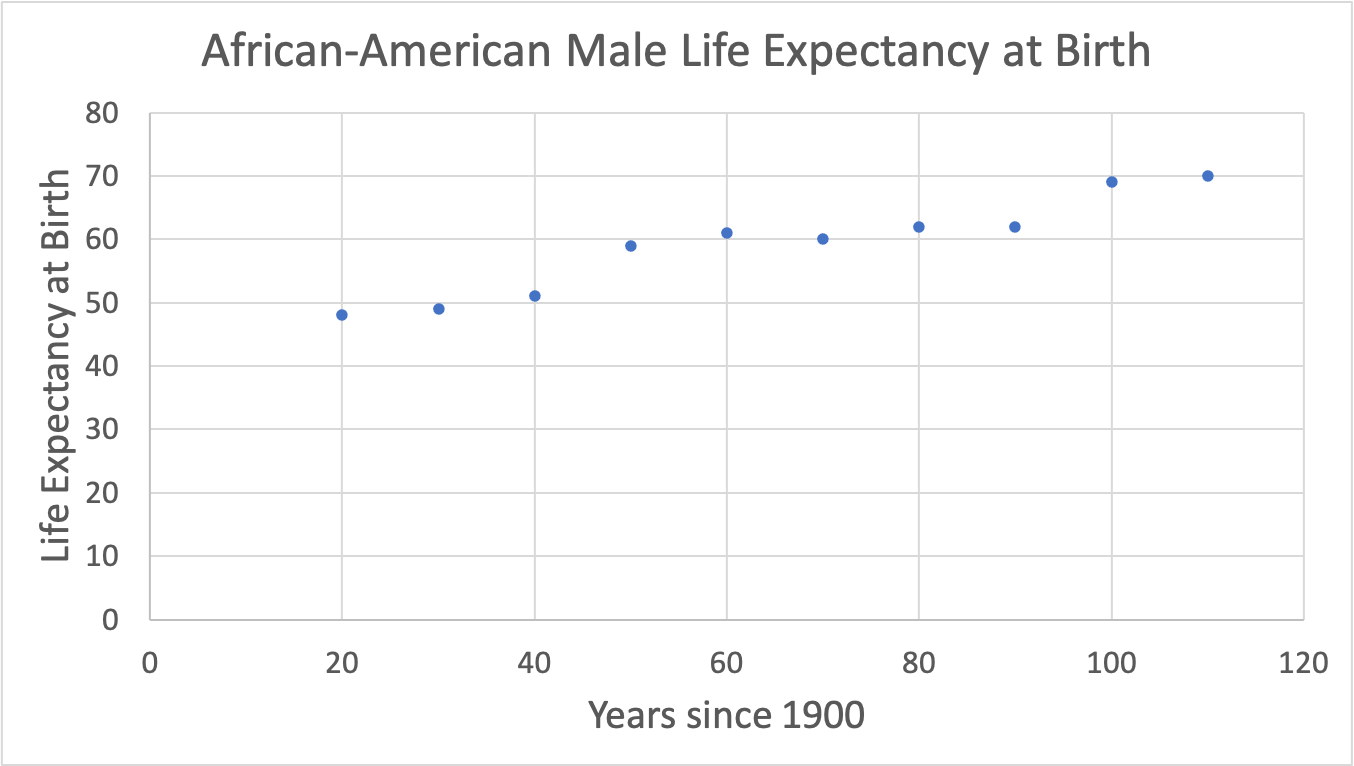
In your group, find a linear model to approximate these data, letting L be the life expectancy at birth and y the year of birth measured in years after 1900. Take a minute to do this individually before discussing your ideas in your group.

(2) In what year will African American male babies have a life expectancy of 75 years? In what year will these male babies be eligible to begin drawing Social Security if the retirement age is raised to 75?

(3) The last part of this collaboration uses data about the life expectancy of a different population of Americans: white females.

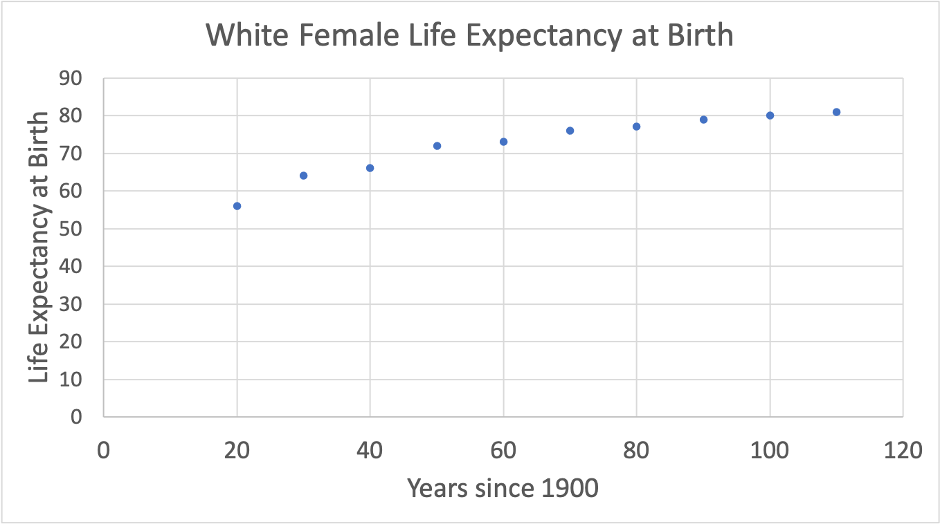
(a) Working with your group, find a linear model to approximate your dataset, letting L be the life expectancy at birth and y the year of birth measured in years after 1900. Be prepared to develop the line you feel best represents the data graphically and how you found the equation of this line.

(b) When does your model predict the population will first have a life expectancy of 75 years at birth? In what year will this group begin collecting Social Security if the retirement age is raised to 75? Be prepared to share your results with the class.

MAKING CONNECTIONS

Record the important mathematical ideas from the discussion.

Search

Text Color

Text Size

Margin Size

Font Type