4.6.2: Exercise 4.6

Last updated
Save as PDF

Page ID: 148779

$ \newcommand{\vecs}[1]{\overset { \scriptstyle \rightharpoonup} {\mathbf{#1}} } $

$ \newcommand{\vecd}[1]{\overset{-\!-\!\rightharpoonup}{\vphantom{a}\smash {#1}}} $

$ \newcommand{\id}{\mathrm{id}}$ $ \newcommand{\Span}{\mathrm{span}}$

( \newcommand{\kernel}{\mathrm{null}\,}\) $ \newcommand{\range}{\mathrm{range}\,}$

$ \newcommand{\RealPart}{\mathrm{Re}}$ $ \newcommand{\ImaginaryPart}{\mathrm{Im}}$

$ \newcommand{\Argument}{\mathrm{Arg}}$ $ \newcommand{\norm}[1]{\| #1 \|}$

$ \newcommand{\inner}[2]{\langle #1, #2 \rangle}$

$ \newcommand{\Span}{\mathrm{span}}$

$ \newcommand{\id}{\mathrm{id}}$

$ \newcommand{\Span}{\mathrm{span}}$

$ \newcommand{\kernel}{\mathrm{null}\,}$

$ \newcommand{\range}{\mathrm{range}\,}$

$ \newcommand{\RealPart}{\mathrm{Re}}$

$ \newcommand{\ImaginaryPart}{\mathrm{Im}}$

$ \newcommand{\Argument}{\mathrm{Arg}}$

$ \newcommand{\norm}[1]{\| #1 \|}$

$ \newcommand{\inner}[2]{\langle #1, #2 \rangle}$

$ \newcommand{\Span}{\mathrm{span}}$ $ \newcommand{\AA}{\unicode[.8,0]{x212B}}$

$ \newcommand{\vectorA}[1]{\vec{#1}} % arrow$

$ \newcommand{\vectorAt}[1]{\vec{\text{#1}}} % arrow$

$ \newcommand{\vectorB}[1]{\overset { \scriptstyle \rightharpoonup} {\mathbf{#1}} } $

$ \newcommand{\vectorC}[1]{\textbf{#1}} $

$ \newcommand{\vectorD}[1]{\overrightarrow{#1}} $

$ \newcommand{\vectorDt}[1]{\overrightarrow{\text{#1}}} $

$ \newcommand{\vectE}[1]{\overset{-\!-\!\rightharpoonup}{\vphantom{a}\smash{\mathbf {#1}}}} $

$ \newcommand{\vecs}[1]{\overset { \scriptstyle \rightharpoonup} {\mathbf{#1}} } $

$ \newcommand{\vecd}[1]{\overset{-\!-\!\rightharpoonup}{\vphantom{a}\smash {#1}}} $

$\newcommand{\avec}{\mathbf a}$ $\newcommand{\bvec}{\mathbf b}$ $\newcommand{\cvec}{\mathbf c}$ $\newcommand{\dvec}{\mathbf d}$ $\newcommand{\dtil}{\widetilde{\mathbf d}}$ $\newcommand{\evec}{\mathbf e}$ $\newcommand{\fvec}{\mathbf f}$ $\newcommand{\nvec}{\mathbf n}$ $\newcommand{\pvec}{\mathbf p}$ $\newcommand{\qvec}{\mathbf q}$ $\newcommand{\svec}{\mathbf s}$ $\newcommand{\tvec}{\mathbf t}$ $\newcommand{\uvec}{\mathbf u}$ $\newcommand{\vvec}{\mathbf v}$ $\newcommand{\wvec}{\mathbf w}$ $\newcommand{\xvec}{\mathbf x}$ $\newcommand{\yvec}{\mathbf y}$ $\newcommand{\zvec}{\mathbf z}$ $\newcommand{\rvec}{\mathbf r}$ $\newcommand{\mvec}{\mathbf m}$ $\newcommand{\zerovec}{\mathbf 0}$ $\newcommand{\onevec}{\mathbf 1}$ $\newcommand{\real}{\mathbb R}$ $\newcommand{\twovec}[2]{\left[\begin{array}{r}#1 \\ #2 \end{array}\right]}$ $\newcommand{\ctwovec}[2]{\left[\begin{array}{c}#1 \\ #2 \end{array}\right]}$ $\newcommand{\threevec}[3]{\left[\begin{array}{r}#1 \\ #2 \\ #3 \end{array}\right]}$ $\newcommand{\cthreevec}[3]{\left[\begin{array}{c}#1 \\ #2 \\ #3 \end{array}\right]}$ $\newcommand{\fourvec}[4]{\left[\begin{array}{r}#1 \\ #2 \\ #3 \\ #4 \end{array}\right]}$ $\newcommand{\cfourvec}[4]{\left[\begin{array}{c}#1 \\ #2 \\ #3 \\ #4 \end{array}\right]}$ $\newcommand{\fivevec}[5]{\left[\begin{array}{r}#1 \\ #2 \\ #3 \\ #4 \\ #5 \\ \end{array}\right]}$ $\newcommand{\cfivevec}[5]{\left[\begin{array}{c}#1 \\ #2 \\ #3 \\ #4 \\ #5 \\ \end{array}\right]}$ $\newcommand{\mattwo}[4]{\left[\begin{array}{rr}#1 \amp #2 \\ #3 \amp #4 \\ \end{array}\right]}$ $\newcommand{\laspan}[1]{\text{Span}\{#1\}}$ $\newcommand{\bcal}{\cal B}$ $\newcommand{\ccal}{\cal C}$ $\newcommand{\scal}{\cal S}$ $\newcommand{\wcal}{\cal W}$ $\newcommand{\ecal}{\cal E}$ $\newcommand{\coords}[2]{\left\{#1\right\}_{#2}}$ $\newcommand{\gray}[1]{\color{gray}{#1}}$ $\newcommand{\lgray}[1]{\color{lightgray}{#1}}$ $\newcommand{\rank}{\operatorname{rank}}$ $\newcommand{\row}{\text{Row}}$ $\newcommand{\col}{\text{Col}}$ $\renewcommand{\row}{\text{Row}}$ $\newcommand{\nul}{\text{Nul}}$ $\newcommand{\var}{\text{Var}}$ $\newcommand{\corr}{\text{corr}}$ $\newcommand{\len}[1]{\left|#1\right|}$ $\newcommand{\bbar}{\overline{\bvec}}$ $\newcommand{\bhat}{\widehat{\bvec}}$ $\newcommand{\bperp}{\bvec^\perp}$ $\newcommand{\xhat}{\widehat{\xvec}}$ $\newcommand{\vhat}{\widehat{\vvec}}$ $\newcommand{\uhat}{\widehat{\uvec}}$ $\newcommand{\what}{\widehat{\wvec}}$ $\newcommand{\Sighat}{\widehat{\Sigma}}$ $\newcommand{\lt}{<}$ $\newcommand{\gt}{>}$ $\newcommand{\amp}{&}$ $\definecolor{fillinmathshade}{gray}{0.9}$

MAKING CONNECTIONS TO THE COLLABORATION

(1) Which of the following was one of the main mathematical ideas of the collaboration?

(i) All exponential models share certain characteristics such as the general shape of the graph, increase or decrease by a percentage, and a vertical intercept.

(ii) Multiplying a number by a second number between 0 and 1 will give you a larger number than you started with.

(iii) Cars lose value quickly after purchase.

(iv) Quarterly compounding happens four times a year.

DEVELOPING SKILLS AND UNDERSTANDING

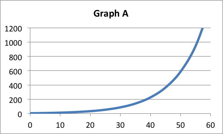
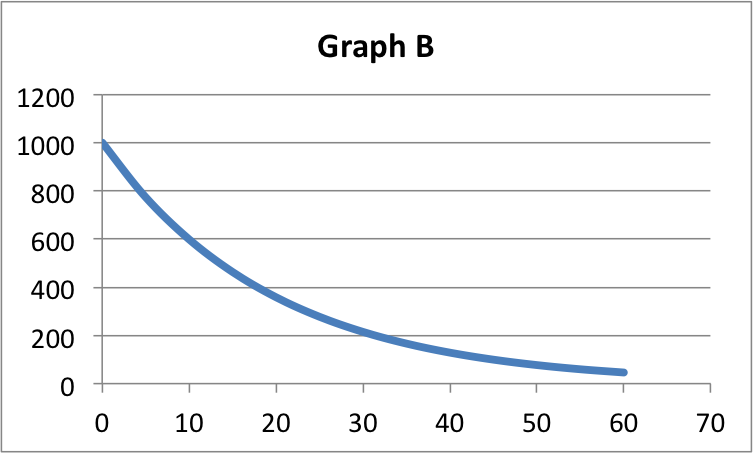
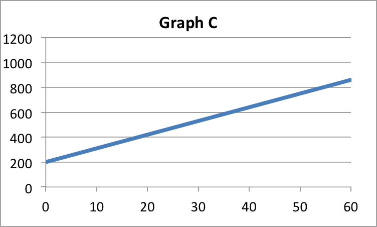
(2) Write the letter of each graph next to the equation that best describes it.

_________ y = 1,000(0.95)^x

_________ y = 200 + 11x

_________ y = 5(1.1)^x

Graph showing an increasing curb, indicating the following:
Start: 0 = 0
End: 60 = 1200 Graph showing a decreasing curb, indicating the following:
Start: 0 = 1,000
End: 60 = just above 0

Graph showing an increasing straight-line, indicating the following:
Start: 0 = 200
End: 60 = just above 800

(3) In this problem, you will compare the effects of different compounding periods on the interest an investment earns. Complete the table below using the values indicated. Show the formula you used, with the correct values, in the second column. The equation used for an annual compounding period has been done for you.

Principal: $1,000
APR: 4.5%
Time: 10 years

Compounding Period	Equation Used for Calculation (with values inserted)	Amount Accrued After 10 Years
Annual	$A = 1000\left( 1 + \dfrac{0.045}{1}\right)^{10\times 1}$	(i)
Quarterly	(ii)	(iii)
Monthly	(iv)	(v)
Daily	(vi)	(vii)

(4) Certain drugs are eliminated from the bloodstream at an exponential rate. Doctors and pharmacists need to know how long it takes for a drug to reach a certain level to determine how often patients should take medications. Answer the following questions about this situation.

(a) Circle the number of the correct statement:

(i) The same amount of the drug will be eliminated in the first hour as in the second hour.

(ii) More of the drug will be eliminated in the first hour than in the second hour.

(iii) Less of the drug will be eliminated in the first hour than in the second hour.

(b) Write an exponential model for the following situation. The drug dosage is 500 mg. The drug is eliminated at a rate of 5.2% per hour. Use D = the amount of the drug in milligrams and t = time in hours. Simplify your answer.

MAKING CONNECTIONS ACROSS THE COURSE

(5) Police officers must investigate the scene of an accident in which a person dies or is severely injured. The police investigators use measurements of skid marks to determine the speed at which the vehicle was traveling at the instant when the driver hit the brakes. The following formula, along with many other factors, is used to estimate the speed of the vehicle:

\[S = \sqrt{30D\cdot f\cdot n}\nonumber \]

where

S = Speed (mph)

30 is a constant value with units of $\dfrac{miles^2}{feet\cdot hour^2}$

D = Skid distance (The skid distance is in feet)

f = Drag factor. The drag factor depends upon the road surface. Portland cement ranges from 0.55 to 1.20, asphalt ranges from 0.50 to 0.90, gravel from 0.40 to 0.80. Units are not used for f.

n = Braking efficiency is quoted as a percent, but used as a decimal. The maximum braking efficiency is 100% (n = 1.00), if all four tires produce skid marks. If the rear brakes were not functioning at all, then n = 0.60. Experts must study the skid marks to determine the appropriate value of n.

(a) Consider the case where a car skids to a stop, leaving four skid marks with an average length of 80 feet. The road is asphalt. Skid tests reveal a drag factor of 0.75. Since all four wheels were braking, the braking efficiency is 100%.

What values should be used for the variables D, f, and n? Fill in the blanks:

D = ________ f = __________ n = ________

Use the formula to estimate the speed of the vehicle (round to the nearest mile per hour).

S = ____________________

(b) Create a table of values for distances of 60, 80, 100, and 120 feet. Round to the nearest mile per hour.

D	S
60	(i)
80	(ii)
100	(iii)
120	(iv)

(d) Is this a linear model? Why or why not?

(e) Is this an exponential model? Why or why not?

Search

Text Color

Text Size

Margin Size

Font Type