8.5: Quantway Core 2.4 Workforce (Health Care) - Student Lesson

Last updated
Save as PDF

Page ID: 148828

\( \newcommand{\vecs}[1]{\overset { \scriptstyle \rightharpoonup} {\mathbf{#1}} } \)

\( \newcommand{\vecd}[1]{\overset{-\!-\!\rightharpoonup}{\vphantom{a}\smash {#1}}} \)

\( \newcommand{\id}{\mathrm{id}}\) \( \newcommand{\Span}{\mathrm{span}}\)

( \newcommand{\kernel}{\mathrm{null}\,}\) \( \newcommand{\range}{\mathrm{range}\,}\)

\( \newcommand{\RealPart}{\mathrm{Re}}\) \( \newcommand{\ImaginaryPart}{\mathrm{Im}}\)

\( \newcommand{\Argument}{\mathrm{Arg}}\) \( \newcommand{\norm}[1]{\| #1 \|}\)

\( \newcommand{\inner}[2]{\langle #1, #2 \rangle}\)

\( \newcommand{\Span}{\mathrm{span}}\)

\( \newcommand{\id}{\mathrm{id}}\)

\( \newcommand{\Span}{\mathrm{span}}\)

\( \newcommand{\kernel}{\mathrm{null}\,}\)

\( \newcommand{\range}{\mathrm{range}\,}\)

\( \newcommand{\RealPart}{\mathrm{Re}}\)

\( \newcommand{\ImaginaryPart}{\mathrm{Im}}\)

\( \newcommand{\Argument}{\mathrm{Arg}}\)

\( \newcommand{\norm}[1]{\| #1 \|}\)

\( \newcommand{\inner}[2]{\langle #1, #2 \rangle}\)

\( \newcommand{\Span}{\mathrm{span}}\) \( \newcommand{\AA}{\unicode[.8,0]{x212B}}\)

\( \newcommand{\vectorA}[1]{\vec{#1}} % arrow\)

\( \newcommand{\vectorAt}[1]{\vec{\text{#1}}} % arrow\)

\( \newcommand{\vectorB}[1]{\overset { \scriptstyle \rightharpoonup} {\mathbf{#1}} } \)

\( \newcommand{\vectorC}[1]{\textbf{#1}} \)

\( \newcommand{\vectorD}[1]{\overrightarrow{#1}} \)

\( \newcommand{\vectorDt}[1]{\overrightarrow{\text{#1}}} \)

\( \newcommand{\vectE}[1]{\overset{-\!-\!\rightharpoonup}{\vphantom{a}\smash{\mathbf {#1}}}} \)

\( \newcommand{\vecs}[1]{\overset { \scriptstyle \rightharpoonup} {\mathbf{#1}} } \)

\( \newcommand{\vecd}[1]{\overset{-\!-\!\rightharpoonup}{\vphantom{a}\smash {#1}}} \)

\(\newcommand{\avec}{\mathbf a}\) \(\newcommand{\bvec}{\mathbf b}\) \(\newcommand{\cvec}{\mathbf c}\) \(\newcommand{\dvec}{\mathbf d}\) \(\newcommand{\dtil}{\widetilde{\mathbf d}}\) \(\newcommand{\evec}{\mathbf e}\) \(\newcommand{\fvec}{\mathbf f}\) \(\newcommand{\nvec}{\mathbf n}\) \(\newcommand{\pvec}{\mathbf p}\) \(\newcommand{\qvec}{\mathbf q}\) \(\newcommand{\svec}{\mathbf s}\) \(\newcommand{\tvec}{\mathbf t}\) \(\newcommand{\uvec}{\mathbf u}\) \(\newcommand{\vvec}{\mathbf v}\) \(\newcommand{\wvec}{\mathbf w}\) \(\newcommand{\xvec}{\mathbf x}\) \(\newcommand{\yvec}{\mathbf y}\) \(\newcommand{\zvec}{\mathbf z}\) \(\newcommand{\rvec}{\mathbf r}\) \(\newcommand{\mvec}{\mathbf m}\) \(\newcommand{\zerovec}{\mathbf 0}\) \(\newcommand{\onevec}{\mathbf 1}\) \(\newcommand{\real}{\mathbb R}\) \(\newcommand{\twovec}[2]{\left[\begin{array}{r}#1 \\ #2 \end{array}\right]}\) \(\newcommand{\ctwovec}[2]{\left[\begin{array}{c}#1 \\ #2 \end{array}\right]}\) \(\newcommand{\threevec}[3]{\left[\begin{array}{r}#1 \\ #2 \\ #3 \end{array}\right]}\) \(\newcommand{\cthreevec}[3]{\left[\begin{array}{c}#1 \\ #2 \\ #3 \end{array}\right]}\) \(\newcommand{\fourvec}[4]{\left[\begin{array}{r}#1 \\ #2 \\ #3 \\ #4 \end{array}\right]}\) \(\newcommand{\cfourvec}[4]{\left[\begin{array}{c}#1 \\ #2 \\ #3 \\ #4 \end{array}\right]}\) \(\newcommand{\fivevec}[5]{\left[\begin{array}{r}#1 \\ #2 \\ #3 \\ #4 \\ #5 \\ \end{array}\right]}\) \(\newcommand{\cfivevec}[5]{\left[\begin{array}{c}#1 \\ #2 \\ #3 \\ #4 \\ #5 \\ \end{array}\right]}\) \(\newcommand{\mattwo}[4]{\left[\begin{array}{rr}#1 \amp #2 \\ #3 \amp #4 \\ \end{array}\right]}\) \(\newcommand{\laspan}[1]{\text{Span}\{#1\}}\) \(\newcommand{\bcal}{\cal B}\) \(\newcommand{\ccal}{\cal C}\) \(\newcommand{\scal}{\cal S}\) \(\newcommand{\wcal}{\cal W}\) \(\newcommand{\ecal}{\cal E}\) \(\newcommand{\coords}[2]{\left\{#1\right\}_{#2}}\) \(\newcommand{\gray}[1]{\color{gray}{#1}}\) \(\newcommand{\lgray}[1]{\color{lightgray}{#1}}\) \(\newcommand{\rank}{\operatorname{rank}}\) \(\newcommand{\row}{\text{Row}}\) \(\newcommand{\col}{\text{Col}}\) \(\renewcommand{\row}{\text{Row}}\) \(\newcommand{\nul}{\text{Nul}}\) \(\newcommand{\var}{\text{Var}}\) \(\newcommand{\corr}{\text{corr}}\) \(\newcommand{\len}[1]{\left|#1\right|}\) \(\newcommand{\bbar}{\overline{\bvec}}\) \(\newcommand{\bhat}{\widehat{\bvec}}\) \(\newcommand{\bperp}{\bvec^\perp}\) \(\newcommand{\xhat}{\widehat{\xvec}}\) \(\newcommand{\vhat}{\widehat{\vvec}}\) \(\newcommand{\uhat}{\widehat{\uvec}}\) \(\newcommand{\what}{\widehat{\wvec}}\) \(\newcommand{\Sighat}{\widehat{\Sigma}}\) \(\newcommand{\lt}{<}\) \(\newcommand{\gt}{>}\) \(\newcommand{\amp}{&}\) \(\definecolor{fillinmathshade}{gray}{0.9}\)

INTRODUCTION

You saw the graph below in Preparation 2.4:

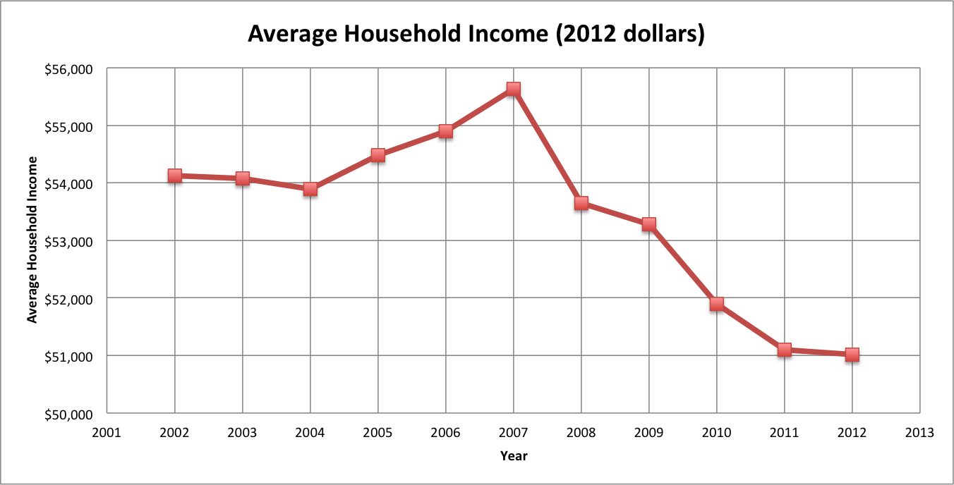
Based on the graph, discuss the following questions in your group:

How much did the Average Household Income increase from 2002 to 2007?
How much did the Average Household Income decrease from 2007 to 2012?

SPECIFIC OBJECTIVES

By the end of this collaboration, you should understand that

the scale on graphs can change the perception of the information they represent.
to fully understand a pie chart, the reference value must be known.

By the end of this collaboration, you should be able to

calculate relative change from a line graph.
estimate the absolute size of the portions of a pie chart given its reference value.
use data displayed on two graphs to estimate a third quantity.

SPECIFIC LANGUAGE AND LITERACY OBJECTIVES

By the end of this collaboration, you should be able to

read and comprehend the problem situation.
read, interpret, and explain the data about trends in obesity in the line graphs.
complete the Double-Entry Journal using information from the problem situation.
demonstrate an understanding of mathematics by writing complete and correct responses to questions.
demonstrate ability to describe, interpret, synthesize, and predict information using the lesson text about diabetes and nutrition.
use appropriate quantitative and health care vocabulary to discuss mathematics in this lesson.

Annotating Problem Situation 1

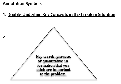
For this collaboration, you will use a skill called annotation. Annotation is a reading comprehension tool that helps you pull out the most important information in a text. In this lesson you will use two types of annotation:

Double-underline the main ideas in the problem situation, and
Draw a triangle around key words, phrases, or quantitative information that you think are important in the problem situation.

Use the annotation symbols in the problem situation below. Your instructor will annotate the first sentence or two with you, as a whole class. Then you will be asked to annotate the remainder of the problem situation on your own as you read.

Image showing the annotation symbols, indicating the following:
- Double-underline key concepts in the problem situation (shown with double lines under this sentence)
- Key words, phrases, or quantitative in formation that you think are important to the problem (shown in a triangle).

PROBLEM SITUATION 1: UNDERSTANDING DIABETES

You are a nurse practitioner and have a new patient named Jane. Jane makes an appointment for a physical examination. You notice in her chart that Jane has gained over 100 pounds (lbs) in the past five years. You run and review some tests on Jane. These tests show that Jane has elevated blood sugar and high blood pressure. She doesn’t have diabetes right now, but you are concerned that she may develop the disease. These tests indicate that she is at high risk for developing diabetes. In addition to diabetes, obesity increases risks of having high blood pressure, heart disease, strokes, cancer, and many other health problems.

Medical professionals think about risk factors that might put patients in danger of having diabetes. Risk factors for diabetes include age, family history of diabetes, high blood pressure, level of physical activity and lifestyle choices, being overweight, and ethnicity.²

You are concerned about Jane because obesity significantly increases the chance a person will develop diabetes. 85.2% of people with type 2 diabetes are overweight. Obesity is increasing in the United States. Approximately 33% of adults and 17% of teens and children in the United States are overweight or obese.³ Figures 1 and 2 below show trends of adult obesity in the United States.

You suggest that Jane should try to lose weight to lower her risk of developing diabetes. Your task is to help Jane understand the link between weight and the high risk of developing diabetes, and to help her make better food and exercise choices to promote weight loss.

Figure 1: Line Graph Depicting Trends of Obesity in the United States

Figure 2: Line Graph Depicting Trends of Obesity in the United States⁴

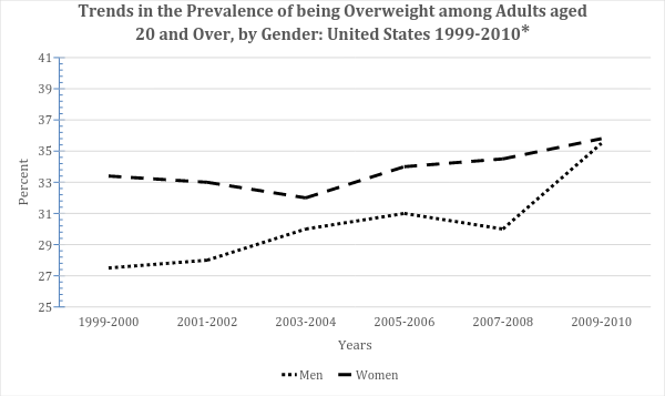
(1) You’ve just read about the link between weight and diabetes. Using Figure 1 and Figure 2, answer the questions below.

(a) Compare the two line graphs about the prevalence of obesity in the United States. To make your comparison, describe how the two graphs are similar and different. What do you notice?

(b) Using the graphs, calculate the relative change in:

(i) the percentage of men who were obese from 1999 to 2010. Round to the nearest whole percent.

(ii) the percentage of women who were obese during the same time period. Round to the nearest whole percent.

(c) Based on your calculations, would you conclude that, in the future, men are more likely to be at risk for developing diabetes than women? Provide support for your answer by connecting quantitative information from the line graphs to the problem situation. Write your answer in 2-3 sentences.

Double-Entry Journal for Problem Situation 2

For the next problem situation, you can use a Double-Entry Journal (DEJ) to help you better understand the details. The DEJ is designed to give you a better understanding of the reading. As you read through Problem Situation 2: Nutrition and Weight Loss, complete the Double-Entry Journal using the steps below.

In the Left Column, list the key ideas or issues in the problem situation.
In the Right Column, write down the key quantitative information in the problem situation.

Key Ideas or Issues in the Problem Situation	Key Quantitative Information In the Problem Situation
1.

PROBLEM SITUATION 2: NUTRITION AND WEIGHT LOSS

As a medical professional, you understand that losing weight can be difficult. You help Jane develop a plan to lose weight. You explain to her that she must monitor her calorie intake. Also, Jane needs to balance the amount of fat, carbohydrates, and proteins in her diet.

For patients trying to lose or maintain weight, doctors recommend that fat should not be more than 35% of a person’s total calorie intake. One way to monitor fat intake is to choose foods with less than 35% of calories from fat. You explain to Jane that 1 gram of fat has 9 calories; 1 gram of protein has 4 calories; and, 1 gram of carbohydrates has 4 calories. Fat contributes the most number of calories per gram. You suggest to Jane that she should limit the amount of fat she eats. Monitoring her fat intake will also help Jane limit the number of calories she consumes.⁵ The problem is that Jane must lose weight. What information does Jane need to make better food choices?

(2) Jane follows a 2000-calorie diet per day.

(a) Use your estimation skills to find Jane’s recommended calorie intake from fat per day.

(b) Calculate the number of grams of fat Jane can consume per day if she follows her diet.

Circle graph showing the Calories that come from Carbohydrates, Protein and Fat in macaroni and cheese.

Fat = 108
Carbs = 124
Protein = 20

Circle graph showing the grams of Carbohydrates, Protein and Fat in macaroni and cheese.

Fat = 12
Carbs = 31
Protein = 5

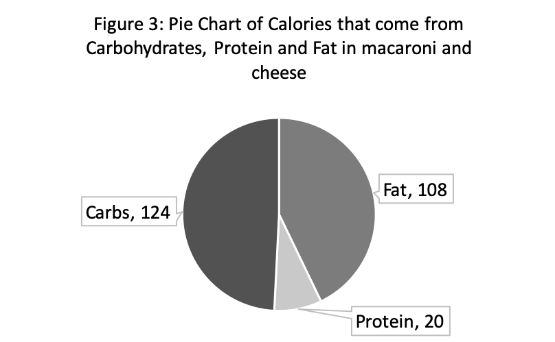
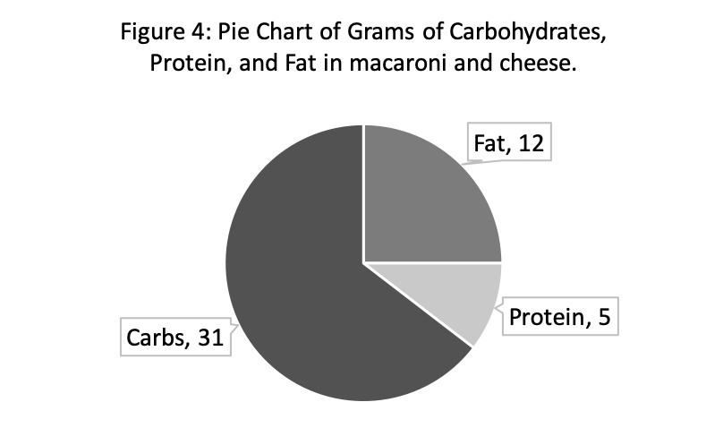
(3) Use the two pie charts above (Figures 3 and 4) to help Jane better understand how to make better food decisions to aid in her weight loss plan. Explain to Jane how the two pie charts look different. Write this explanation in 1-2 complete sentences. It is important to write complete sentences because it helps your instructor better understand your mathematical thinking.

(4) (a) According to the pie graphs shown above, does the percent of calories from fat in macaroni and cheese exceed the recommended amount of 35%?

(b) Based on your answer above, can Jane eat one serving of macaroni and cheese per day and still satisfy the overall daily guidelines for fat content? Explain why or why not?

(c) How many servings of macaroni and cheese could Jane eat per day and still stay within the recommended guidelines for the amount of dietary fat she should consume?

PROBLEM SITUATION 3: INTERPRETING BAR GRAPHS—MAKING HEALTHY FOOD CHOICES

Your task is to help Jane understand how to make healthier food choices. Jane must understand why monitoring fat intake is important when trying to lose weight. Each gram of fat contains more calories than each gram of carbohydrates or protein. Therefore, eating a lot of fat can increase calorie intake significantly.

The following two bar graphs below represent four food products and the fat content in each product. Help Jane understand which products would best support weight loss.

Figure 5: Bar Graph of Fat Grams in Food Products⁶	Figure 6: Bar Graph of Percent of Calories from Fat in Food Products⁷

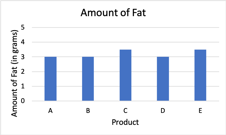
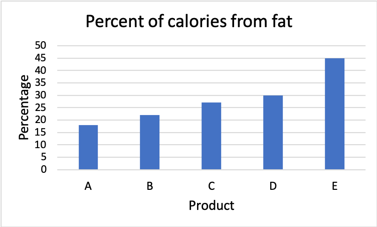
(5) Think about the statement, “Food items A, B, and D have the same number of grams of fat, but the products have different percentages of fat content.”

(a) How can this be true? Write your answer in 1-2 complete sentences.

(b) Which products would you recommend to someone who is trying to lose weight, and why? Remember, one way to monitor fat intake is to choose foods with less than 35% of calories from fat.

(6) Let’s imagine a new product is released: Product F. Product F has 3.7 grams of fat and it contains 140 calories.

(a) Calculate the percent of calories in Product F that come from fat. Round to the nearest whole percent.

(b) Would you recommend this product for someone trying to lose weight? Explain.

FURTHER APPLICATIONS

(7) Using the information from the bar graphs in Figures 5 and 6, determine how many calories are in Product D? (Remember: There are 9 calories per 1 gram of fat).

MAKING CONNECTIONS

Record the important mathematical ideas from the discussion. When thinking about what the important ideas were from the discussion, think about today’s objectives for the collaboration. Also think about the problem context.

________________________________________

² http://www.diabetes.org/diabetes-basics/?loc=db-slabnav

³ http://professional.diabetes.org/admin/UserFiles/0%20-%20Sean/FastFacts%20March%202013.pdf

⁴ http://www.cdc.gov/nchs/data/hestat/obese/obese99.htm

⁵ http://www.mckinley.illinois.edu/handouts/macronutrients.htm

⁶ http://nutritiondata.self.com/

⁷ http://nutritiondata.self.com/