3.3: Simulation of Population Growth

Last updated
Save as PDF

Page ID: 93504

$ \newcommand{\vecs}[1]{\overset { \scriptstyle \rightharpoonup} {\mathbf{#1}} } $ $ \newcommand{\vecd}[1]{\overset{-\!-\!\rightharpoonup}{\vphantom{a}\smash {#1}}} $$\newcommand{\id}{\mathrm{id}}$ $ \newcommand{\Span}{\mathrm{span}}$ $ \newcommand{\kernel}{\mathrm{null}\,}$ $ \newcommand{\range}{\mathrm{range}\,}$ $ \newcommand{\RealPart}{\mathrm{Re}}$ $ \newcommand{\ImaginaryPart}{\mathrm{Im}}$ $ \newcommand{\Argument}{\mathrm{Arg}}$ $ \newcommand{\norm}[1]{\| #1 \|}$ $ \newcommand{\inner}[2]{\langle #1, #2 \rangle}$ $ \newcommand{\Span}{\mathrm{span}}$ $\newcommand{\id}{\mathrm{id}}$ $ \newcommand{\Span}{\mathrm{span}}$ $ \newcommand{\kernel}{\mathrm{null}\,}$ $ \newcommand{\range}{\mathrm{range}\,}$ $ \newcommand{\RealPart}{\mathrm{Re}}$ $ \newcommand{\ImaginaryPart}{\mathrm{Im}}$ $ \newcommand{\Argument}{\mathrm{Arg}}$ $ \newcommand{\norm}[1]{\| #1 \|}$ $ \newcommand{\inner}[2]{\langle #1, #2 \rangle}$ $ \newcommand{\Span}{\mathrm{span}}$$\newcommand{\AA}{\unicode[.8,0]{x212B}}$

As we have seen, stochastic modeling is significantly more complicated than deterministic modeling. As the modeling becomes more sophisticated, a numerical simulation becomes necessary. Here, for illustration, we show how to simulate individual realizations of population growth.

A naive approach would make use of the birth rate $b$ directly. During the short time interval $\Delta t$, each individual has probability $b \Delta t$ of giving birth. We can decide if an individual gives birth by generating a random deviate (a pseudo-random number between zero and one): if the random deviate is less than $b \Delta t$, then the individual gives birth; if larger than $b \Delta t$, then the individual does not. With $N$ individuals at time $t$, we then simply compute $N$ random deviates. Counting the number of random deviates less than $b \Delta t$ allows us to update the population size to the time $t+\Delta t$. For accuracy, $\Delta t$ must be small, making this a computationally slow method.

There is, however, a much more efficient way to simulate population growth. Define a random variable $\tau=\tau(N)$ to be the time it takes for a population to grow from size $N$ to size $N+1$ because of a single birth. The random variable $\tau$ is called the interevent time and represents the elapsed time between births. A simulation from population size $N_{0}$ to size $N_{f}$ would then simply require computing $N_{f}-N_{0}$ different random values of $\tau$, a relatively easy and quick computation if we know the probability density function (pdf) of $\tau$.

Accordingly, we define $P(\tau)$ to be the pdf of $\tau$ for a population of size $N$. The cumulative distribution function (cdf), $F(\tau)$, defined as the probability that the interevent time is less that $\tau$ is given by

\[F(\tau)=\int_{0}^{\tau} P(\tau) d \tau \nonumber \]

where $P(\tau)=F^{\prime}(\tau)$. The complementary cumulative distribution function (ccdf), $G(\tau)$, defined as the probability that the interevent time is greater than $\tau$ is given by $G(\tau)=1-F(\tau)$

Now the probability that the interevent time is greater than $\tau+\Delta \tau$, with $\Delta \tau$ small, is given by the probability that it is greater than $\tau$ times the probability that there are no births in the time interval $\Delta \tau$. Therefore, $G(\tau+\Delta \tau)$ satisfies

\[G(\tau+\Delta \tau)=G(\tau)(1-b N \Delta \tau) \nonumber \]

Differencing $G$ and taking the limit $\Delta \tau \rightarrow 0$ yields the differential equation

\[\frac{d G}{d \tau}=-b N G \nonumber \]

which can be integrated using the initial condition $G(0)=1$ to obtain

\[G(\tau)=e^{-b N \tau} \nonumber \]

From $G(\tau)$, we can find

\[F(\tau)=1-e^{-b N \tau}, \quad P(\tau)=b N e^{-b N \tau} \nonumber \]

The pdf, $P(\tau)$, has the form of an exponential distribution with parameter $b N$.

Here, we make use of a well-known result from probability theory that enables us to compute $\tau$ using random deviates. With $y$ a random deviate, $\tau$ can be computed from $\tau=F^{-1}(y)$, where $F^{-1}$ is the inverse function of $F .$ The correct formula for the exponential distribution is

\[\tau=-\frac{\ln (1-y)}{b N} \nonumber \]

To simulate a population growing from $N_{0}$ to $N_{f}$, we compute $N_{f}-N_{0}$ random deviates $y$, and then compute the corresponding interevent times using $(3.3.6)$, taking care to adjust the population size $N$ as the population grows.

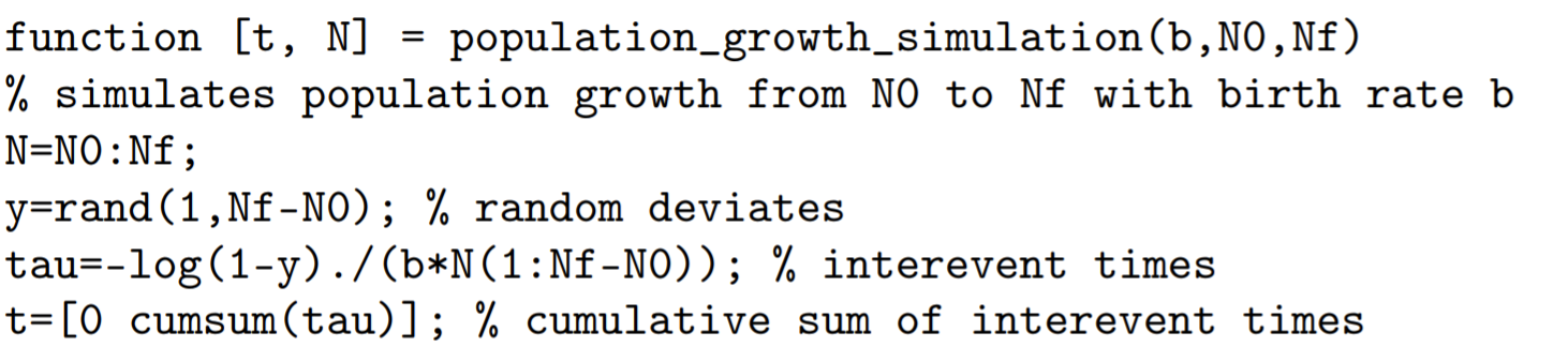
Below, we illustrate a simple MATLAB function that simulates one realization of population growth from initial size $N_{0}$ to final size $N_{f}$, with birth rate $b$.

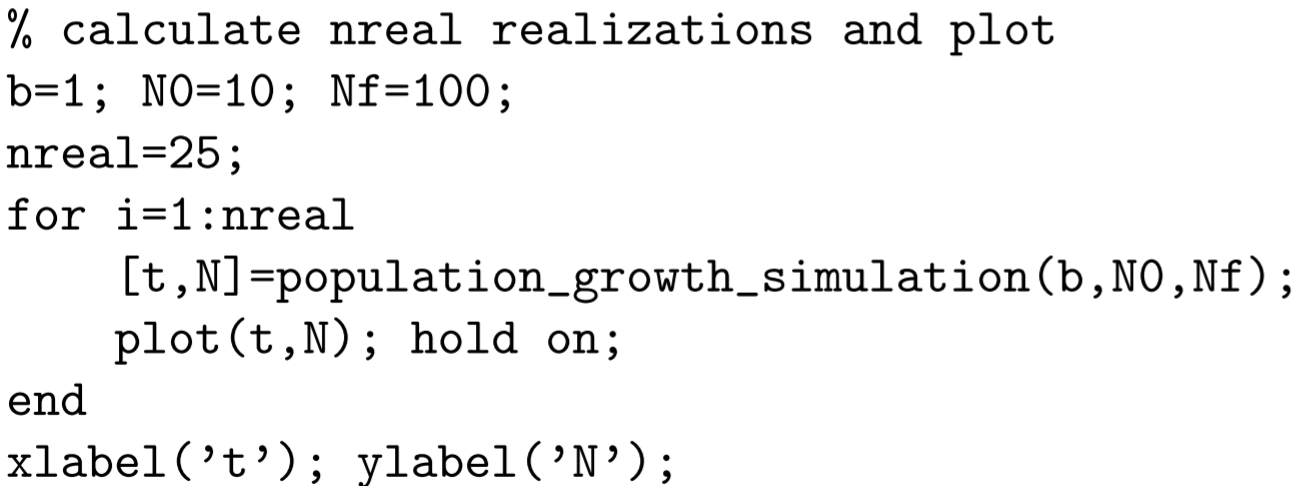
$clipboard_efdf560ad98aa12e8df103c9f2207bd79.png$

The function population_growth_simulation.m can be driven by a MATLAB script to compute realizations of population growth. For instance, the following script computes 25 realizations for a population growth from 10 to 100 with $b=1$ and plots all the realizations:

Figure $3.1$ presents three graphs, showing 25 realizations of population growth starting with population sizes of 10,100 , and 1000 , and ending with population sizes a factor of 10 larger. Observe that the variance, relative to the initial population size, decreases as the initial population size increases, following our analytical result (3.31). (a)

Figure 3.1: Twenty-five realizations of population growth with initial population sizes of 10,100 , and 1000 , in (a), (b), and (c), respectively.