4.3: The SIR Epidemic Disease Model
- Page ID
- 93507

\( \newcommand{\vecs}[1]{\overset { \scriptstyle \rightharpoonup} {\mathbf{#1}} } \)
\( \newcommand{\vecd}[1]{\overset{-\!-\!\rightharpoonup}{\vphantom{a}\smash {#1}}} \)
\( \newcommand{\dsum}{\displaystyle\sum\limits} \)
\( \newcommand{\dint}{\displaystyle\int\limits} \)
\( \newcommand{\dlim}{\displaystyle\lim\limits} \)
\( \newcommand{\id}{\mathrm{id}}\) \( \newcommand{\Span}{\mathrm{span}}\)
( \newcommand{\kernel}{\mathrm{null}\,}\) \( \newcommand{\range}{\mathrm{range}\,}\)
\( \newcommand{\RealPart}{\mathrm{Re}}\) \( \newcommand{\ImaginaryPart}{\mathrm{Im}}\)
\( \newcommand{\Argument}{\mathrm{Arg}}\) \( \newcommand{\norm}[1]{\| #1 \|}\)
\( \newcommand{\inner}[2]{\langle #1, #2 \rangle}\)
\( \newcommand{\Span}{\mathrm{span}}\)
\( \newcommand{\id}{\mathrm{id}}\)
\( \newcommand{\Span}{\mathrm{span}}\)
\( \newcommand{\kernel}{\mathrm{null}\,}\)
\( \newcommand{\range}{\mathrm{range}\,}\)
\( \newcommand{\RealPart}{\mathrm{Re}}\)
\( \newcommand{\ImaginaryPart}{\mathrm{Im}}\)
\( \newcommand{\Argument}{\mathrm{Arg}}\)
\( \newcommand{\norm}[1]{\| #1 \|}\)
\( \newcommand{\inner}[2]{\langle #1, #2 \rangle}\)
\( \newcommand{\Span}{\mathrm{span}}\) \( \newcommand{\AA}{\unicode[.8,0]{x212B}}\)
\( \newcommand{\vectorA}[1]{\vec{#1}} % arrow\)
\( \newcommand{\vectorAt}[1]{\vec{\text{#1}}} % arrow\)
\( \newcommand{\vectorB}[1]{\overset { \scriptstyle \rightharpoonup} {\mathbf{#1}} } \)
\( \newcommand{\vectorC}[1]{\textbf{#1}} \)
\( \newcommand{\vectorD}[1]{\overrightarrow{#1}} \)
\( \newcommand{\vectorDt}[1]{\overrightarrow{\text{#1}}} \)
\( \newcommand{\vectE}[1]{\overset{-\!-\!\rightharpoonup}{\vphantom{a}\smash{\mathbf {#1}}}} \)
\( \newcommand{\vecs}[1]{\overset { \scriptstyle \rightharpoonup} {\mathbf{#1}} } \)
\(\newcommand{\longvect}{\overrightarrow}\)
\( \newcommand{\vecd}[1]{\overset{-\!-\!\rightharpoonup}{\vphantom{a}\smash {#1}}} \)
\(\newcommand{\avec}{\mathbf a}\) \(\newcommand{\bvec}{\mathbf b}\) \(\newcommand{\cvec}{\mathbf c}\) \(\newcommand{\dvec}{\mathbf d}\) \(\newcommand{\dtil}{\widetilde{\mathbf d}}\) \(\newcommand{\evec}{\mathbf e}\) \(\newcommand{\fvec}{\mathbf f}\) \(\newcommand{\nvec}{\mathbf n}\) \(\newcommand{\pvec}{\mathbf p}\) \(\newcommand{\qvec}{\mathbf q}\) \(\newcommand{\svec}{\mathbf s}\) \(\newcommand{\tvec}{\mathbf t}\) \(\newcommand{\uvec}{\mathbf u}\) \(\newcommand{\vvec}{\mathbf v}\) \(\newcommand{\wvec}{\mathbf w}\) \(\newcommand{\xvec}{\mathbf x}\) \(\newcommand{\yvec}{\mathbf y}\) \(\newcommand{\zvec}{\mathbf z}\) \(\newcommand{\rvec}{\mathbf r}\) \(\newcommand{\mvec}{\mathbf m}\) \(\newcommand{\zerovec}{\mathbf 0}\) \(\newcommand{\onevec}{\mathbf 1}\) \(\newcommand{\real}{\mathbb R}\) \(\newcommand{\twovec}[2]{\left[\begin{array}{r}#1 \\ #2 \end{array}\right]}\) \(\newcommand{\ctwovec}[2]{\left[\begin{array}{c}#1 \\ #2 \end{array}\right]}\) \(\newcommand{\threevec}[3]{\left[\begin{array}{r}#1 \\ #2 \\ #3 \end{array}\right]}\) \(\newcommand{\cthreevec}[3]{\left[\begin{array}{c}#1 \\ #2 \\ #3 \end{array}\right]}\) \(\newcommand{\fourvec}[4]{\left[\begin{array}{r}#1 \\ #2 \\ #3 \\ #4 \end{array}\right]}\) \(\newcommand{\cfourvec}[4]{\left[\begin{array}{c}#1 \\ #2 \\ #3 \\ #4 \end{array}\right]}\) \(\newcommand{\fivevec}[5]{\left[\begin{array}{r}#1 \\ #2 \\ #3 \\ #4 \\ #5 \\ \end{array}\right]}\) \(\newcommand{\cfivevec}[5]{\left[\begin{array}{c}#1 \\ #2 \\ #3 \\ #4 \\ #5 \\ \end{array}\right]}\) \(\newcommand{\mattwo}[4]{\left[\begin{array}{rr}#1 \amp #2 \\ #3 \amp #4 \\ \end{array}\right]}\) \(\newcommand{\laspan}[1]{\text{Span}\{#1\}}\) \(\newcommand{\bcal}{\cal B}\) \(\newcommand{\ccal}{\cal C}\) \(\newcommand{\scal}{\cal S}\) \(\newcommand{\wcal}{\cal W}\) \(\newcommand{\ecal}{\cal E}\) \(\newcommand{\coords}[2]{\left\{#1\right\}_{#2}}\) \(\newcommand{\gray}[1]{\color{gray}{#1}}\) \(\newcommand{\lgray}[1]{\color{lightgray}{#1}}\) \(\newcommand{\rank}{\operatorname{rank}}\) \(\newcommand{\row}{\text{Row}}\) \(\newcommand{\col}{\text{Col}}\) \(\renewcommand{\row}{\text{Row}}\) \(\newcommand{\nul}{\text{Nul}}\) \(\newcommand{\var}{\text{Var}}\) \(\newcommand{\corr}{\text{corr}}\) \(\newcommand{\len}[1]{\left|#1\right|}\) \(\newcommand{\bbar}{\overline{\bvec}}\) \(\newcommand{\bhat}{\widehat{\bvec}}\) \(\newcommand{\bperp}{\bvec^\perp}\) \(\newcommand{\xhat}{\widehat{\xvec}}\) \(\newcommand{\vhat}{\widehat{\vvec}}\) \(\newcommand{\uhat}{\widehat{\uvec}}\) \(\newcommand{\what}{\widehat{\wvec}}\) \(\newcommand{\Sighat}{\widehat{\Sigma}}\) \(\newcommand{\lt}{<}\) \(\newcommand{\gt}{>}\) \(\newcommand{\amp}{&}\) \(\definecolor{fillinmathshade}{gray}{0.9}\)The SIR model, first published by Kermack and McKendrick in 1927, is undoubtedly the most famous mathematical model for the spread of an infectious disease. Here, people are characterized into three classes: susceptible \(S\), infective \(I\) and removed R. Removed individuals are no longer susceptible nor infective for whatever reason; for example, they have recovered from the disease and are now immune, or they have been vaccinated, or they have been isolated from the rest of the population, or perhaps they have died from the disease. As in the SIS model, we assume that infectives leave the \(I\) class with constant rate \(\gamma\), but in the SIR model they move directly into the \(R\) class. The model may be diagrammed as
\[S \stackrel{\beta S I}{\longrightarrow} I \stackrel{\gamma I}{\longrightarrow} R, \nonumber \]
and the corresponding coupled differential equations are
\[\frac{d S}{d t}=-\beta S I, \quad \frac{d I}{d t}=\beta S I-\gamma I, \quad \frac{d R}{d t}=\gamma I, \nonumber \]
with the constant population constraint \(S+I+R=N\). For convenience, we nondimensionalize (4.3.2) using \(N\) for population size and \(\gamma^{-1}\) for time; that is, let
\[\hat{S}=S / N, \quad \hat{I}=I / N, \quad \hat{R}=R / N, \quad \hat{t}=\gamma t \nonumber \]
and define the dimensionless basic reproductive ratio as
\[\mathcal{R}_{0}=\frac{\beta N}{\gamma} \nonumber \]
The dimensionless SIR equations are then given by
\[\frac{d \hat{S}}{d \hat{t}}=-\mathcal{R}_{0} \hat{S} \hat{I}, \quad \frac{d \hat{I}}{d \hat{t}}=\mathcal{R}_{0} \hat{S} \hat{I}-\hat{I}, \quad \frac{d \hat{R}}{d \hat{t}}=\hat{I}, \nonumber \]
with dimensionless constraint \(\hat{S}+\hat{I}+\hat{R}=1\).
We will use the SIR model to address two fundamental questions: (1) Under what condition does an epidemic occur? (2) If an epidemic occurs, what fraction of a well-mixed population gets sick?
Let \(\left(\hat{S}_{*}, \hat{I}_{*}, \hat{R}_{*}\right)\) be the fixed points of (4.3.5). Setting \(d \hat{S} / d \hat{t}=d \hat{I} / d \hat{t}=d \hat{R} / d \hat{t}=0\), we immediately observe from the equation for \(d \hat{R} / d \hat{t}\) that \(\hat{I}=0\), and this value forces all the time-derivatives to vanish for any \(\hat{S}\) and \(\hat{R}\). Since with \(\hat{I}=0\), we have \(\hat{R}=1-\hat{S}\), evidently all the fixed points of (4.3.5) are given by the one parameter family \(\left(\hat{S}_{*}, \hat{I}_{*}, \hat{R}_{*}\right)=\left(\hat{S}_{*}, 0,1-\hat{S}_{*}\right) .\)
An epidemic occurs when a small number of infectives introduced into a susceptible population results in an increasing number of infectives. We can assume an initial population at a fixed point of \((4.3.5)\), perturb this fixed point by introducing a small number of infectives, and determine the fixed point’s stability. An epidemic occurs when the fixed point is unstable. The linear stability problem may be solved by considering only the equation for \(d \hat{I} / d \hat{t}\) in (4.3.5). With \(\hat{I} \ll 1\) and \(\hat{S} \approx \hat{S}_{0}\), we have
\[\frac{d \hat{I}}{d \hat{t}}=\left(\mathcal{R}_{0} \hat{S}_{0}-1\right) \hat{I} \nonumber \]
so that an epidemic occurs if \(\mathcal{R}_{0} \hat{S}_{0}-1>0\). With the basic reproductive ratio given by (4.3.4), and \(S_{0}=S_{0} / N\), where \(S_{0}\) is the number of initial susceptible individuals, an epidemic occurs if
\[\mathcal{R}_{0} \hat{S}_{0}=\frac{\beta S_{0}}{\gamma}>1 \nonumber \]
which could have been guessed. An epidemic occurs if an infective individual introduced into a population of \(S_{0}\) susceptible individuals infects on average more than one other person. If an epidemic occurs, then initially the number of infective individuals increases exponentially with growth rate \(\beta S_{0}-\gamma\).
which upon integration and simplification, results in the following transcendental equation for \(\hat{R}_{\infty}\) :
\[1-\hat{R}_{\infty}-e^{-\mathcal{R}_{0} \hat{R}_{\infty}}=0, \nonumber \]
an equation that can be solved numerically using Newton’s method. We have
\[\begin{aligned} &F\left(\hat{R}_{\infty}\right)=1-\hat{R}_{\infty}-e^{-\mathcal{R}_{0} \hat{R}_{\infty}} \\[4pt] &F^{\prime}\left(\hat{R}_{\infty}\right)=-1+\mathcal{R}_{0} e^{-\mathcal{R}_{0} \hat{R}_{\infty}} \end{aligned} \nonumber \]
and Newton’s method for solving \(F\left(\hat{R}_{\infty}\right)=0\) iterates
\[\hat{R}_{\infty}^{(n+1)}=\hat{R}_{\infty}^{n}-\frac{F\left(\hat{R}_{\infty}^{(n)}\right)}{F^{\prime}\left(\hat{R}_{\infty}^{(n)}\right)} \nonumber \]
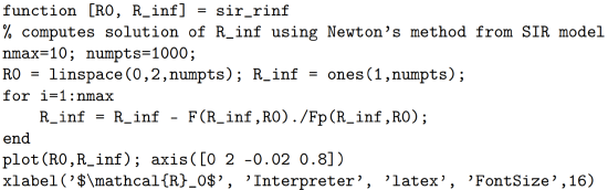
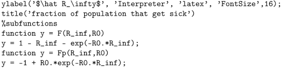
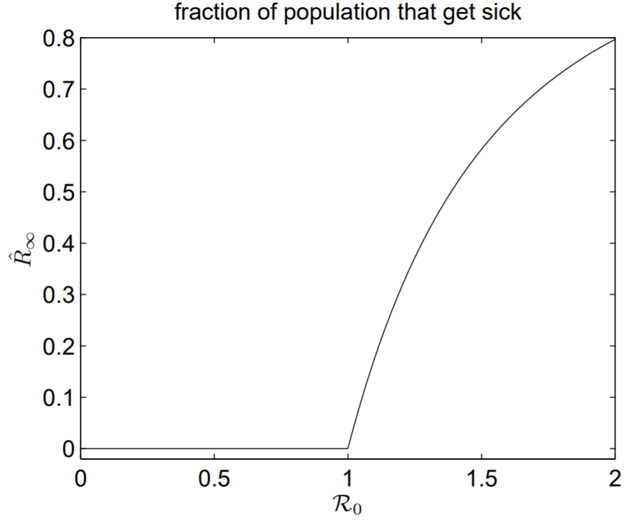
for fixed \(\mathcal{R}_{0}\) and a suitable initial condition for \(R_{\infty}^{(0)}\), which we take to be unity. My code for computing \(R_{\infty}\) as a function of \(\mathcal{R}_{0}\) is given below, and the result is shown in Fig. 4.1. There is an explosion in the number of infections as \(\mathcal{R}_{0}\) increases from unity, and this rapid increase is a classic example of what is known more generally as a threshold phenomenon.