1.3: Galois Connections

The preservation of meets and joins, and in particular issues concerning generative effects, is tightly related to the theory of Galois connections, which is a special case of a more general theory we will discuss later, namely that of adjunctions. We will use some adjunction terminology when describing Galois connections.

Definition and examples of Galois connections

Galois connections between preorders were first considered by Évariste Galois who didn’t call them by that name in the context of a connection he found between “field extensions” and “automorphism groups.” We will not discuss this further, but the idea is that given two preorders P and Q, a Galois connection is a pair of maps back and forth from P to Q and from Q to P with certain properties, which make it like a relaxed version of isomorphisms. To be a bit more precise, preorder isomorphisms are examples of Galois connections, but Galois connections need not be preorder isomor- phisms.

Definition: 1.95.

A Galois connection between preorders P and Q is a pair of monotone maps f : P→Q and g :Q→P such that

f(p) ≤ q if and only if p ≤ g(q). (1.96)

We say that f is the left adjoint and g is the right adjoint of the Galois connection.

Example 1.97.

Consider the map (3×−): \(\mathbb{Z}\) → \(\mathbb{R}\) which sends x \(\in\) \(\mathbb{Z}\) to 3x, which we can consider as a real number 3x \(\in\) \(\mathbb{Z}\) \(\subseteq\) \(\mathbb{R}\).

Let’s find a left adjoint for the map (3 × −).

Write ⌈z⌉ for the smallest natural number above z \(\in\) \(\mathbb{R}\), and write ⌊z⌋ for the largest integer below z \(\in\) R, e.g. ⌈3.14⌉= 4 and ⌊3.14⌋ = 3.\(^{a}\) As the left adjoint \(\mathbb{R}\) → \(\mathbb{Z}\), let’s see if ⌈−/3⌉ works.

It is easily checked that

⌈x/3⌉ ≤ y if and only if x ≤ 3y.

Success! Thus we have a Galois connection between ⌈−/3⌉ and (3 × −).

\(^{a}\)By “above” and “below,” we mean greater than or equal to or less than or equal to; the latter being a mouthful. Anyway, ⌊3⌋ = 3 = ⌈3⌉.

Exercise 1.98.

In Example 1.97 we found a left adjoint for the monotonemap (3×−): \(\mathbb{Z}\)→ \(\mathbb{R}\). Now find a right adjoint for the same map, and show it is correct. ♦

Exercise 1.99.

Consider the preorder P = Q = 3.

1. Let f , g be the monotone maps shown below:

Is it the case that f is left adjoint to g? Check that for each 1 ≤ p, q ≤ 3, one has f (p) ≤ q iff p ≤ g(q).

2. Let f , g be the monotone maps shown below:

3. Is it the case that f is left adjoint to g? ♦

Remark 1.100. The pictures in Exercise 1.99 suggest the following idea. If P and Q are total orders and f : P → Q and g : Q → P are drawn with arrows bending counter- clockwise, then f is left adjoint to g iff the arrows do not cross. With a little bit of thought, this can be formalised. We think this is a pretty neat way of visualizing Galois connections between total orders!

Exercise 1.101.

1. Does ⌈−/3⌉ have a left adjoint L :\(\mathbb{Z}\) → \(\mathbb{R}\)?
2. If not, why? If so, does its left adjoint have a left adjoint?

Back to partitions

Recall from Example 1.52 that we can understand the set Prt(S) of partitions on a set S in terms of surjective functions out of S.

Suppose we are given any function g : S → T. We will show that this function g induces a Galois connection \(g_{!}: \operatorname{Prt}(S) \leftrightarrows \operatorname{Prt}(T): g^{*}\), between preorder of S-partitions and the preorder of T-partitions. The way you might explain it to a seasoned category theorist is:

The left adjoint is given by taking any surjection out of S and pushing out along g to get a surjection out of T. The right adjoint is given by taking any surjection out of T, composing with g to get a function out of S, and then taking the epi-mono factorization to get a surjection out of S.

By the end of this book, the reader will understand pushouts and epi-mono factorizations, so he or she will be able to make sense of the above statement. But for now we will explain the process in more down-to-earth terms.

Start with g : S → T; we first want to understand g! : Prt(S) → Prt(T). So start with a partition \(_{∼S}\) of S. To begin the process of obtaining a partition \(_{∼T}\) on T, say that two elements \(t_{1}\), \(t_{2}\) \(\in\) T are in the same part, \(t_{1}\) \(_{∼T}\) \(t_{2}\), if there exist \(s_{1}\), \(s_{2}\) \(\in\) S with such that \(s_{1}\) ∼s \(s_{2}\) and g(\(s_{1}\)) = \(t_{1}\) and g(s2) = \(t_{2}\). However, the result of doing so will not necessarily be transitive you may get \(t_{1}\) ∼T \(t_{2}\) and \(t_{2}\) ∼T \(t_{3}\) without \(t_{1} \sim_{T}^{?} t_{3}-\) and partitions must be transitive. So complete the process by just adding in the missing pieces (take the transitive closure). The result is g!(∼S) := \(_{∼T}\). Again starting with g, we want to get the right adjoint g∗: Prt(T) → Prt(S). So start with a partition \(_{∼T}\) of T. Get a partition \(_{∼S}\) on S by saying that \(s_{1}\) \(_{∼S}\) \(s_{2}\) iff g(\(s_{1}\)) \(_{∼T}\) g(\(s_{2}\)). The result is g*(\(_{~T}\)) := \(_{~S}\).

Example 1.102.

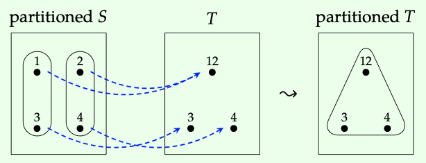
Let S = {1,2,3,4}, T = {12,3,4}, and g: S → T by g(1) := g(2) := 12, g(3) := 3, and g(4) := 4. The partition shown left below is translated by \(g_{!}\) to the partition shown on the right.

Exercise 1.103.

There are 15 different partitions of a set with four elements. Choose 6 different ones and for each one, call it c: S --» P, find g!(c), where S, T,

and g: S → T are the same as they were in Example 1.102. ♦

Example 1.104.

Let S, T be as below, and let g: S → T be the function shown in blue. Here is a picture of how \(g^{∗}\) takes a partition on T and “pulls it back” to a partition on S:

Exercise 1.105.

There are five partitions possible on a set with three elements, say T = {12,3,4}. Using the same S and g : S → T as in Example 1.102, determine the partition \(g^{∗}\)(c) on S for each of the five partitions c: T --» P. ♦

To check that for any function g: S → T, the monotone map \(g_{!}\): Prt(S) → Prt(T) really is left adjoint to \(g^{∗}\): Prt(T) → Prt(S) would take too much time for this sketch. But the following exercise gives some evidence.

Exercise 1.106.

Let S, T, and g: S → T be as in Example 1.102.

1. Choose a nontrivial partition c : S --» P and let \(g_{!}\)(c) be its push forward partition on T.
2. Choose any coarser partition d : T --» P′, i.e. where \(g_{!}\)(c) ≤ d.
3. Choose any non-coarser partition e: T --» Q, i.e. where \(g_{!}\)(c) \(\nleq\) e. (If you can’t do this, revise your answer for #1.)
4. Find \(g^{∗}\)(d) and \(g^{∗}\)(e).
5. The adjunction formula Eq. (1.96) in this case says that since \(g_{!}\)(c) ≤ d and \(g_{!}\)(c) \(\nleq\) e, we should have c ≤ \(g^{∗}\)(d) and c \(\nleq\) \(g^{∗}\)(e). Show that this is true. ♦

Basic theory of Galois connections

Proposition 1.107

Suppose that f : P → Q and g : Q → P are monotone maps. The following are equivalent

f and g form a Galois connection where f is left adjoint to g,

(b) for every p \(\in\) P and q \(\in\) Q we have

p ≤ g(f(p)) and f(g(q)) ≤ q. (1.108)

Proof. Suppose f is left adjoint to g. Take any p \(\in\) P, and let q := f (p). By reflexivity, we have f (p) ≤ q, so by the Definition 1.95 of Galois connection we have p ≤ g(q), but this means p ≤ g( f (p)). The proof that f (g(q)) ≤ q is similar.

Now suppose that Eq. (1.108) holds for all p ∈ P and q ∈ Q. We want show that f(p) ≤ q iff p ≤ g(q). Suppose f(p) ≤ q; then since g is monotonic, g(f(p)) ≤ g(q), but p ≤ g(f(p)) so p ≤ g(q). The proof that p ≤ g(q) implies f(p) ≤ q is similar. □

Exercise 1.109.

Complete the proof of Proposition 1.107 by showing that

1. if f is left adjoint to g then for any q \(\in\) Q, we have f(g(q)) ≤ q, and
2. if Eq. (1.108) holds, then holds p ≤ g(q) iff f(p) ≤ q holds, for all p \(\in\) P and q \(\in\) Q. ♦

If we replace ≤ with = in Eq. (1.108), we get back the definition of isomorphism (Definition 1.75); this is why we said at the beginning of Section 1.4.1 that Galois connections are a kind of relaxed version of isomorphisms.

Exercise 1.110.

1. Show that if f : P → Q has a right adjoint g, then it is unique up to isomorphism. That means, for any other right adjoint g′, we have g(q) \(\cong\) g′(q) for all q \(\in\) Q.
2. Is the same true for left adjoints? That is, if h: P → Q has a left adjoint, is it necessarily unique up to isomorphism? ♦

Proposition 1.111 (Right adjoints preserve meets).

Let f : P → Q be left adjoint to g:Q→P. Suppose A \(\subseteq\) Q any subset, and let g(A) := {g(a) | a \(\in\) A} be its image. Then if A has a meet \(\bigwedge\)A \(\in\) Q then g(A) has a meet \(\bigwedge\)g(A) in P, and we have

g(\(\bigwedge A)\) \(\cong\) \(\bigwedge\)g(A).

That is, right adjoints preserve meets. Similarly, left adjoints preserve joins: if A \(\subseteq\) P is any subset that has a join VA \(\in\) P, then f(A) has a join Vf(A) in Q, and we have

f(V A) \(\cong\) V f(A).

Proof. Let f : P → Q and g: Q → P be adjoint monotone maps, with g right adjoint to f . Let A \(\subseteq\) Q be any subset and let m := \(bigwedge\)A be its meet. Then since g is monotone g(m) ≤ g(a) for all a \(\in\) A, so g(m) is a lower bound for the set g(A). We will be done if we can show g(m) is a greatest lower bound. So take any other lower bound b for g(A); that is suppose that for all a \(\in\) A, we have b ≤ g(a) and we want to show b ≤ g(m). Then by definition of g being a right adjoint (Definition 1.95), we also have f (b) ≤ a. This means that f (b) is a lower bound for A in Q. Since the meet m is the greatest lower bound, we have f (b) ≤ m. Once again using the Galois connection, b ≤ g(m), proving that g(m) is indeed the greatest lower bound for g(A), as desired.

The second claim is proved similarly; see Exercise 1.112.

Exercise 1.112.

Complete the proof of Proposition 1.111 by showing that left adjoints preserve joins. ♦

Since left adjoints preserve joins, we know that they cannot have generative effects. In fact, we will see in Theorem 1.115 that a monotone map does not have generative effects—i.e. it preserves joins—if and only if it is a left adjoint to some other monotone.

Example 1.113.

Right adjoints need not preserve joins. Here is an example:

Let g be the map that preserves labels, and let f be the map that preserves labels as far as possible but with f (3.9) := 4. Both are f and g monotonic, and one can check that g is right adjoint to f (see Exercise 1.114). But g does not preserve joins because 1 \(\lor\) 2 = 4 holds in Q, whereas g(1) \(\lor\) g(2) = 1 \(\lor\) 2 = 3.9 \(\neq\) 4 = g(4) in P.

Exercise 1.114.

To be sure that g really is right adjoint to f in Example 1.113, there are twelve tiny things to check; do so. That is, for every p \(\in\) P and q \(\in\) Q, check that f (p) ≤ q iff p ≤ g(q). ♦

Theorem 1.115 (Adjoint functor theorm for preorders).

Suppose Q is a preorder that has all meets and let P be any preorder. A monotone map g : Q → P preserves meets if and only if it is a right adjoint.

Similarly, if P has all joins and Q is any preorder, a monotone map f : P → Q preserves joins if and only if it is a left adjoint.

Proof. We will only prove the claim about meets; the claim about joins follows similarly. We proved one direction in Proposition 1.111, namely that right adjoints preserve meets. For the other, suppose that g is a monotone map that preserves meets; we shall construct a left adjoint f .

We define our candidate f : P → Q on any p \(\in\) P by

f(p) := \(\bigwedge\){q \(\in\) Q | p \(\leq\) g(q)}; (1.116)

this meet is well defined because Q has all meets, but for f to really be a candidate, we need to show it is monotone. So suppose that p ≤ p′. Then {q′ \(\in\) Q | p′ ≤ g(q′)} \(\subseteq\) {q \(\in\) Q | p ≤ g(q)}. By Proposition 1.91, this implies f (p) ≤ f (p′). Thus f is monotone.

By Proposition 1.111, it suffices to show that \(p_{0}\) ≤ g(f (\(p_{0}\))) and that f (g(\(q_{0}\))) ≤ \(q_{0}\) for all \(p_{0}\) \(\in\) P and \(q_{0}\) \(\in\) Q. For the first, we have

\(p_{0}\) \(\leq\) \(\bigwedge\){g(q) \(\in\) P | \(p_{0}\) \(\leq\) g(q)} \(\cong\) g(\(\bigwedge\){q \(\in\) Q | \(p_{0}\) \(\leq\) g(q)}) = g(f(\(p_{0}\)),

where the first inequality follows from the fact that if \(p_{0}\) is below every element of a set, then it is below their meet, and the isomorphism is by definition of g preserving meets. For the second, we have

f(g(\(q_{0}\)) = \(\bigwedge\){q \(\in\) Q | g(\(q_{0}\)) \(\leq\) g(q)} \(\leq\) \(\bigwedge\){\(q_{0}\)} = \(q_{0}\),

where the first inequality follows from Proposition 1.91 since {\(q_{0}\)} \(\subseteq\) {q \(\in\) Q | g(\(q_{0}\)) ≤ g(q)}, and the fact that \(\bigwedge\){\(q_{0}\)} = \(q_{0}\). □

Example 1.117.

Let f : A → B be a function between sets. We can imagine A as a set of apples, B as a set of buckets, and f as putting each apple in a bucket.

Then we have the monotone map \(f^{∗}\) : P(Y) → P(X) that category theorists call “pullback along f .” This map takes a subset B′ \(\subseteq\) B to its preimage \(f^{ −1}\)(B′) \(\subseteq\) A: that is, it takes a collection B′ of buckets, and tells you all the apples that they contain in total. This operation is monotonic (more buckets means more apples) and it has both a left and a right adjoint. The left adjoint \(f_{!}\)(A) is given by the direct image: it maps a subset A′ \(\subseteq\) A to

\(f_{!}\)(A') := {b \(\in\) B | there exists a \(\in\) A' such that f(a) = b}

This map takes a set A′ of apples, and tells you all the buckets that contain at least one of those apples.

The right adjoint \(f^{∗}\) maps a subset A′ \(\subseteq\) A to

\(f_{*}\)(A') := {b \(\in\) B | for all a such that f(a) = b, we have a \(\in\) A'}

This map takes a set A′ of apples, and tells you all the buckets b that are all A′: all the apples in b are from the chosen subset A′. Note that if a bucket doesn’t contain any apples at all, then vacuously all its apples are from A′, so empty buckets count as far as \(f_{∗}\) is concerned.

Notice that all three of these operations turn out to be interesting: start with a set B′ of buckets and return all the apples in them, or start with a set A′ of apples and either find the buckets that contain at least one apple from A′, or the buckets whose only apples are from A′. But we did not invent these mappings \(f_{∗}\), \(f_{!}\), and \(f_{∗}\): they were induced by the function f . They were automatic. It is one of the pleasures of category theory that adjoints so often turn out to have interesting semantic interpretations.

Exercise 1.118.

Choose sets X and Y with between two and four elements each, and choose a function f : X → Y.

1. Choose two different subsets B1, B2 \(\subseteq\) Y and find \(f^{∗}\)(B1) and \(f^{∗}\)(B2).
2. Choose two different subsets A1, A2 \(\subseteq\) X and find \(f_{!}\)(A1) and \(f_{!}\)(A2).
3. With the same A1, A2 \(\subseteq\) X, find \(f_{∗}\)(A1) and \(f_{∗}\)(A2). ♦

Closure operators

Given a Galois connection with f : P → Q left adjoint to g: Q → P, we may compose f and g to arrive at a monotonemap f :P → P from preorder P to itself. This monotone map has the property that p ≤ (f ; g)(p), and that (f ; g ; f ; g)(p) \(\cong\) (f ; g)(p) for any p \(\in\) P. This is an example of a closure operator.

Exercise 1.119.

Suppose that f is left adjoint to g. Use Proposition 1.107 to show the following.

1. p ≤ (f ; g)(p).
2. (f ; g ; f ; g)(p) \(\cong\) (f ; g)(p). To prove this, show inequalities in both directions, ≤ and ≥. ♦

Definition: 1.120.

A closure operator j : P → P on a preorder P is a monotone map such that for all p \(\in\) P we have

(a) p ≤ j(p);
(b) j(j(p)) \(\cong\) j(p).

Example 1.121.

Here is an example of closure operators from computation, very roughly presented. Imagine computation as a process of rewriting input expressions to output expressions. For example, a computer can rewrite the expression 7+2+3 as the expression 12. The set of arithmetic expressions has a partial order according to whether one expression can be rewritten as another.

We might think of a computer program, then, as a method of taking an expression and reducing it to another expression. So it is a map j : exp → exp. It furthermore is desirable to require that this computer program is a closure operator. Monotonicity means that if an expression x can be rewritten into expression y, then the reduction j(x) can be rewritten into j(y). Moreover, the requirement x ≤ j(x) implies that j can only turn one expression into another if doing so is a permissible rewrite. The requirement

j(j(x)) = j(x) implies if you try to reduce an expression that has already been reduced, the computer program leaves it as is. These properties provide useful structure in the analysis of program semantics.

Example 1.122 (Adjunctipms from closure operators).

Just as every adjunction gives rise to a closure operator, from every closure operator we may construct an adjunction.

Let P be a preorder and let j : P → P be a closure operator. We can define a preorder \(fix_{j}\) to have elements the fixed points of j; that is,

\(fix_{j}\) := {p \(\in\) P | j(p) \(\cong\) p}.

This is a subset of P, and inherits an order as a result; hence \(fix_{j}\) is a sub-preorder of P. Note that j(p) is a fixed point for all p \(\in\) P, since j(j(p)) \(\cong\) j(p).

We define an adjunction with left adjoint j: P → \(fix_{j}\) sending p to j(p), and right adjoint g: \(fix_{j}\) → P simply the inclusion of the sub-preorder. To see it’s really an adjunction, we need to see that for any p \(\in\) P and q \(\in\) \(fix_{j}\), we have j(p) ≤ q if and only if p ≤ q. Let’s check it. Since p ≤ j(p), we have that j(p) ≤ q implies p ≤ q by transitivity. Conversely, since q is a fixed point, p ≤ q implies j(p) ≤ j(q) \(\cong\) q.

Example 1.123.

Another example of closure operators comes from logic. This will be discussed in the final chapter of the book, in particular Section 7.4.5, but we will give a quick overview here. In essence, logic is the study of when one formal statement or proposition implies another. For example, if n is prime then n is not a multiple of 6, or if it is raining then the ground is getting wetter. Here “n is prime”, “n is not a multiple of 6”, “it is raining”, and “the ground is getting wetter” are propositions, and we gave two implications. Take the set of all propositions, and order them by p ≤ q iff p implies q, denoted p ⇒ q. Since p ⇒ p and since whenever p ⇒ q and q ⇒ r, we also have p ⇒ r, this is indeed a preorder.

A closure operator on it is often called a modal operator. It is a function j from propositions to propositions, for which p ⇒ j(p) and j(j(p)) = j(p). An example of a j is “assuming Bob is in San Diego....” Think of this as a proposition B; so “assuming Bob is in San Diego, p” means B ⇒ p. Let’s see why B ⇒ − is a closure operator. If ‘p’ is true then “assuming Bob is in San Diego, p” is still true. Suppose that “assuming Bob is in San Diego it is the case that, assuming Bob is in San Diego, p’ is true.” It follows that “assuming Bob is in San Diego, p” is true. So we have seen, at least informally, that “assuming Bob is in San Diego...” is a closure operator.

Level shifting

The last thing we want to discuss in this chapter is a phenomenon that happens often in category theory, something we might informally call “level-shifting.” It is easier to give an example of this than to explain it directly.

Given any set S, there is a set Rel(S) of binary relations on S. An element R \(\in\) Rel(S) is formally a subset R \(\subseteq\) S × S. The set Rel(S) can be given an order via the subset relation, R \(\subseteq\) R′, i.e. if whenever R(\(_{s1}\), \(_{s2}\)) holds then so does R′(\(_{s1}\), \(_{s2}\)).

For example, the Hasse diagram for Rel({1}) is:

Exercise 1.124.

Draw the Hasse diagram for the preorder Rel({1, 2}) of all binary relations on the set {1, 2}. ♦

For any set S, there is also a set Pos(S), consisting of all the preorder relations on S. In fact there is a preorder structure \(\sqsubseteq\) on Pos(S), again given by inclusion: ≤ is below ≤′ (we’ll write ≤\(\sqsubseteq\)≤′) if a ≤ b implies a ≤′ b for every a, b \(\in\) S. A preorder of preorder structures? That’s what we mean by a level shift.

Every preorder relation is in particular a relation, so we have an inclusion Pos(S) → Rel(S). This is the right adjoint of a Galois connection.

Its left adjoint is a monotone map Cl: Rel(S) → Pos(S) given by taking any relation R, writing it in infix notation using ≤, and taking the reflexive and transitive closure, i.e. adding s ≤ s for every s and adding s ≤ u whenever s ≤ t and t ≤ u.

Exercise 1.125.

Let S = {1, 2, 3}. Let’s try to understand the adjunction discussed above.

1. Come up with any preorder relation ≤ on S, and define U(≤) to be the subset U(≤) := {(s1,s2) | s1 ≤ s2} \(\subseteq\) S×S, i.e. U(≤) is the image of ≤ under the inclusion Pos(S) → Rel(S), the relation ‘underlying’ the preorder.

2. Come up with any two binary relations Q \(\subseteq\) S×SandQ′ \(\subseteq\) S×S such that Q \(\subseteq\) U(≤) but Q′ \(\nsubseteq\) U(≤). Note that your choice of Q, Q′ do not have to come from preorders.

We now want to check that in this case, the closure operation Cl is really left adjoint to the ‘underlying relation’ map U.

3. Concretely (without using the assertion that there is some sort of adjunction), show that Cl(Q) \(\sqsubseteq\) ≤, where \(\sqsubseteq\) is the order on Pos(S), defined immediately above this exercise.

4. Concretely show that Cl(Q′) \(\not\sqsubseteq\) ≤. ♦