2.5: Computing presented V-categories with matrix mult

In Section 2.3.3 we promised a straightforward way to construct the matrix representa- tion of a Cost-category from a Cost-weighted graph. To do this, we use a generalized matrix multiplication. We shall show that this works, not just for Cost, but also for Bool, and many other monoidal preorders. The property required of the preorder is that of being a unital, commutative quantale. These are preorders with all joins, plus one additional ingredient, being monoidal closed, which we define next, in Section 2.5.1. The definition of a quantale will be given in Section 2.5.2

Monoidal closed preorders

The definition of V-category makes sense for any symmetric monoidal preorder V. But that does not mean that any base of enrichment V is as useful as any other. In this section we define closed monoidal categories, which in particular enrich themselves! “Before you can really enrich others, you should really enrich yourself.”

Definition: Word

A symmetric monoidal preorder V = (V, ≤, I, ⊗) is called symmetric monoidal closed (or just closed) if, for every two elements v, w \(\in\) V, there is an element v = w in V, called the hom-element, with the property

(a ⊗ v) ≤w iff a ≤ (v −o w). (2.80)

for all a, v, w \(\in\) V.

Remark 2.81. The term ‘closed’ refers to the fact that a hom-element can be constructed for any two elements, so the preorder can be seen as closed under the operation of “taking homs.” In later chapters we’ll meet the closely-related concepts of compact closed categories (Definition 4.58) and cartesian closed categories (Section 7.2.1) that make this idea more precise. See especially Exercise 7.11.

One can consider the hom-element v −o w as a kind of “single-use v-to-w converter.” So Eq. (2.80) says that a and v are enough to get w if and only if a is enough to get a single-use v-to-w converter.

Exercise 2.82.

Condition Eq. (2.80) says precisely that there is a Galois connection in the sense of Definition 1.95. Let’s prove this fact. In particular, we’ll prove that a monoidal preorder is monoidal closed iff, given any v \(\in\) V, the map (− ⊗ v): V → V given by multiplying with v has a right adjoint. We write this right adjoint (v −o−): V → V.

1. Using Definition 2.2, show that (− ⊗ v) is monotone.
2. Supposing that V is closed, show that for all v, w \(\in\) V we have ((v −o w) ⊗v) ≤ w.
3. Using 2., show that (v −o−) is monotone.
4. Conclude that a symmetric monoidal preorder is closed if and only if the monotone map (− ⊗ v) has a right adjoint. ♦

Example 2.83.

The monoidal preorder Cost = ([0, ∞], ≥, 0, +) is monoidal closed. Indeed, for any x, y \(\in\) [0, ∞], define x −o y := max(0, y − x). Then, for any a, x, y \(\in\) [0, ∞], we have

a + x ≥ y iff a ≥ y − x iff max(0,a) ≥ max(0, y−x) iff a ≥ (x −o y)

so −o satisfies the condition of Eq. (2.80).
Note that we have not considered subtraction in Cost before; we can in fact use monoidal closure to define subtraction in terms of the order and monoidal structure!

Exercise 2.84.

Show that Bool = (\(\mathbb{B}\), ≤, true, \(\land\)) is monoidal closed. ♦

Example 2.85.

A non-example is (\(\mathbb{B}\), ≤, false, \(\lor\)). Indeed, suppose we had a −o operator as in Definition 2.79. Note that false ≤ p −o q, for any p, q no matter what −o is, because false is less than everything. But using a = false, p = true, and q = false, we then get a contradiction: (a ∨ p) \(\nleq\) q and yet a ≤ (p −o q).

Example 2.86.

We started this chapter talking about resource theories. What does the closed structure look like from that perspective? For example, in chemistry it would say that for every two material collections c, d one can form a material collection c −o d with the property that for any a, one has

a + c → d if and only if a → (c −o d).

Or more down to earth, since we have the reaction 2\(H_{2}\)O + 2Na → 2NaOH + \(H_{2}\), we must also have

2\(H_{2}\)O → (2Na −o (2NaOH + \(H_{2}\)))

So from just two molecules of water, you can form a certain substance, and not many

substances fit the bill—our preorder Mat of chemical materials is not closed.

But it is not so far-fetched: this hypothetical new substance (2Na −o (2NaOH + \(H_{2}\))) is not really a substance, but a potential reaction: namely that of converting a sodium to sodium-hydroxide-plus-hydrogen. Two molecules of water unlock that potential.

Proposition 2.87.

Suppose V = (V, ≤, I, ⊗, −o) is a symmetric monoidal preorder that is closed. Then

(a) For every v \(\in\) V, the monotone map − ⊗ v: (V,≤) → (V,≤) is left adjoint to v −o −: (V, ≤) → (V, ≤).

(b) For any element v \(\in\) V and set of elements A \(\subseteq\) V, if the join \(\bigvee\)\(_{a \in\ A}\)a \(\in\) A a exists then so does a \(\in\) A v ⊗ a and we have

\(\left(v \otimes \bigvee_{a \in A} a\right) \cong \bigvee_{a \in A}(v \otimes a)\) (2.88)

(c) Foranyv, w \(\in\) V, we have v ⊗(v −o w) ≤ w.

(d) For any v \(\in\)V, we havev \(\cong\) (I −o v).

(e) For any u, v, w \(\in\)V, we have (u −o v) ⊗ (v −o w) ≤ (u −o w).

Proof. We go through the claims in order.

(a) The definition of (− ⊗ v) being left adjoint to (v −o) is exactly the condition Eq. (2.80); see Definition 1.95 and Exercise 2.82.

(b) This follows from (a), using the fact that left adjoints preserve joins (Proposition 1.111).

(c) This follows from (a), using the equivalent characterisation of Galois connection in Proposition 1.107. More concretely, from reflexivity (v −o w) ≤ (v −o w), we obtain (v −o w) ⊗ v ≤ w Eq. (2.80), and we are done by symmetry, which says v ⊗ (v −o w) = (v −o w) ⊗ v.

(d) Since v ⊗ I = v ≤ v, Eq.(2.80) says v ≤ (I −o v). For the other direction, we have (I −o v) = I ⊗ (I −o v) ≤ v by (c).

(e)To obtain this inequality, we just need u ⊗ (u −o v) ⊗ (v −o w) ≤ w. But this follows by two applications of (c). □

One might read (c) as saying “if I have a v and a single-use v-to-w converter, I can have a w.” One might read (d) as saying “having a v is the same as having a single-use nothing-to-v converter.” And one might read (e) as saying “if I have a single-use u-to-v converter and a single-use v-to-w converter, I can get a single-use u-to-w converter.

Remark 2.89. We can consider V to be enriched in itself. That is, for every v, w \(\in\) Ob(V), we can define V(v, w) := (v −o w) \(\in\) V. For this to really be an enrichment, we just need to check the two conditions of Definition 2.46. The first condition I ≤ X(x, x) = (x −o x) is satisfied because I ⊗ x ≤ x. The second condition is satisfied by Proposition 2.87(e).

Quantales

To perform matrix multiplication over a monoidal preorder, we need one more thing: joins. These were first defined in Definition 1.81.

Definition: 2.90.

A unital commutative quantale is a symmetric monoidal closed preorder V = (V, ≤, I, ⊗, −o) that has all joins: \(\bigvee\)A exists for every \(\bigvee\)A \(\subseteq\) V. In particular, we often denote the empty join by 0 := \(\bigvee\) Ø.

Whenever we speak of quantales in this book, we mean unital commutative quantales. We will try to remind the reader of that. There are also very interesting applications of noncommutative quantales; see Section 2.6.

Example 2.91.

In Example 2.83, we saw that Cost is monoidal closed. To check whether Cost is a quantale, we take an arbitrary set of elements A \(\subseteq\) [0, ∞] and ask if it has a join \(\bigvee\)A. To be a join, it needs to satisfy two properties:

a. a ≥ \(\bigvee\)A for all a \(\in\) A, and

b. if b \(\in\) [0,∞] is any element such that a ≥ b for all a \(\in\) A, then \(\bigvee\)A ≥ b. In fact we can define such a join: it is typically called the infimum, or greatest lower bound, of A.\(^{5}\) For example, if A = {2, 3} then \(\bigvee\)A = 2. We have joins for infinite sets too: if B = {2.5, 2.05, 2.005, . . .}, its infimum is 2. Finally, in order to say that ([0, ∞], ≥) has all joins, we need a join to exist for the empty set A = Ø too. The first condition becomes vacuous there are no a’s in A but the second condition says that for any b \(\in\) [0, ∞] we have \(\bigvee\)Ø ≥ b; this means \(\bigvee\)Ø = ∞.

Thus indeed ([0, ∞], ≥) has all joins, so Cost is a quantale.

Exercise 2.92.

1. What is \(\bigvee\)Ø, which we generally denote 0, in the case

a. V = Bool = (\(\mathbb{B}\), ≤, true, \(\wedge\))?

b. V = Cost = ([0,∞], ≥, 0, +)?

2. What is the join x \(\lor\) y in the case

a. V = Bool, and x, y \(\in\) \(\mathbb{B}\) are booleans?

b. V = Cost, and x, y \(\in\) [0,∞] are distances? ♦

Exercise 2.93.

Show that Bool = (\(\mathbb{B}\), ≤, true, \(\wedge\)) is a quantale. ♦

Exercise 2.94.

Let S be a set and recall the power set monoidal preorder (P(S), \(\subseteq\), S, \(\land\)) from Exercise 2.35. Is it a quantale? ♦

Remark 2.95. One can personify the notion of unital, commutative quantale as a kind of navigator. A navigator is someone who understands “getting from one place to an- other.” Different navigators may care about or understand different aspects—whether one can get from A to B, how much time it will take, what modes of travel will work, etc. but they certainly have some commonalities. Most importantly, a navigator needs to be able to read a map: given routes A to B and B to C, they understand how to get a route A to C. And they know how to search over the space of way-points to get from A to C. These will correspond to the monoidal product and the join operations, respectively.

Proposition 2.96.

Let P = (P, ≤) be a preorder. It has all joins iff it has all meets.

Proof. The joins (resp. meets) in P are the meets (resp. joins) in \(P^{op}\), so the two claims are dual: it suffices to show that if P has all joins then it has all meets.

Suppose P has all joins and suppose that A \(\subseteq\) P is a subset for which we want themeet. Consider the set \(M_{A}\) := {p \(\in\) P | p ≤ a for all a \(\in\) A} of elements below everything in A. Let \(m_{A}\) := \(\bigvee\)\(_{p \in\ M}\)\(_{A}\) p be their join. We claim that \(M_{A}\) is a meet for A. We first need to know that for any a \(\in\) A we have \(m_{A}\) ≤ a, but this is by definition of join: since all p \(\in\) \(M_{A}\) satisfy p ≤ a, so does their join \(m_{A}\) ≤ a. We second need to know that for any m′ \(\in\) P with m′ ≤ a for all a \(\in\) A, we have m′ ≤ m. But every such m′ is actually an element of \(M_{A}\) and m is their join, so m′ ≤ m. This completes the proof. □

In particular, a quantale has all meets and all joins, even though we only define it to have all joins.

Remark 2.97. The notion of Hausdorff distance can be generalized, allowing the role of Cost to be taken by any quantale V. If X is a V-category with objects X, and U \(\subseteq\) X and V (\subseteq\) X, we can generalize the usual Hausdorff distance, on the left below, to the formula on the right:

\(\begin{equation}
d(U, V):=\sup _{u \in U} \inf _{v \in V} d(u, v) \quad x(U, V):=\bigwedge_{u \in U} \bigvee_{v \in V} X(u, v)
\end{equation}\)

For example, if V = Bool, the Hausdorff distance between sub-preorders U and V answers the question “can I get into V from every u \(\in\) U,” i.e. \(\forall{u}\) \(\in\) U . \(\exists{v}\) \(\in\) V . u ≤ v. Or for another example, use V = P(M) with its interpretation as modes of transportation, as in Exercise 2.62. Then the Hausdorff distance d(U, V) \(\in\) P(M) tells us those modes of transportation that will get us into V from every point in U.

Proposition 2.98.

Suppose V = (V, ≤, I, ⊗) is any symmetric monoidal preorder that has all joins. Then V is closed—i.e. it has a −o operation and hence is a quantale if and only if ⊗ distributes over joins; i.e. if Eq. (2.88) holds for all v \(\in\) V and A \(\subseteq\) V.

Proof. We showed one direction in Proposition 2.87(b): if V is monoidal closed then Eq. (2.88) holds. We need to show that Eq. (2.88) holds then − ⊗ v : V → V has a right adjoint v −o−. This is just the adjoint functor theorem, Theorem 1.115. It says we can define v −o w to be

\(\begin{equation} v −o w:=\bigvee_{\{a \in V \mid a \otimes v \leq w\}} a \end{equation}\) □

Matrix multiplication in a quantale

A quantale V = (V, ≤, I, ⊗, −o), as defined in Definition 2.79, provides what is necessary to perform matrix multiplication.\(^{6}\) The usual formula for matrix multiplication is:

\(\begin{equation} (M * N)(i, k)=\sum_{j} M(i, j) * N(j, k) \end{equation}\). (2.99)

We will get a formula where joins stand in for the sum operation \(\sigma\), and ⊗ stands in for the product operation ∗. Recall our convention of writing 0 := \(\bigvee\).

Definition: 2.100.

Let V = (V, ≤, ⊗, I) be a quantale. Given sets X and Y, a matrix with entries in V, or simply a V-matrix, is a function M:X × Y → V. For any x \(\in\) X and y \(\in\) Y, we call M(x, y) the (x, y)-entry.

Here is how you multiply V-matrices M: X × Y → V and N: Y × Z → V. Their product is defined to be the matrix (M ∗ N): X × Z → V, whose entries are given by the formula

\(\begin{equation} (M * N)(x, z):=\bigvee_{y \in Y} M(x, y) \otimes N(y, z) \end{equation}\) (2.101)

Note how similar this is to Eq. (2.99).

Example 2.102.

Let V = Bool. Here is an example of matrix multiplication M ∗ N. Here X = {1, 2, 3}, Y = {1, 2}, and Z = {1, 2, 3}, matrices M : X × Y → \(\mathbb{B}\) and N : Y × Z → \(\mathbb{B}\) are shown to the left below, and their product is shown to the right:

The identity V-matrix on a set X is \(I_{X}\) : X × X → V given by

\(\begin{equation}
I_{X}(x, y):=\left\{\begin{array}{ll}
I & \text { if } x=y \\
0 & \text { if } x \neq y
\end{array}\right.
\end{equation}\)

Exercise 2.103

Write down the 2×2-identity matrix for each of the quantales (\(\mathbb{N}\), ≤, 1, ∗), Bool = (\(mathbb{B}\), ≤, true, \(\wedge\)), and Cost = ([0, ∞], ≥, 0, +).

Exercise 2.104

Let V = (V, ≤, I, ⊗, −o) be a quantale. Use Eq. (2.101) and Proposition 2.87 to prove the following.

1. Prove the identity law: for any sets X and Y and V-matrix M: X × Y → V, one has IX ∗ M = M.
2. Prove the associative law: for any matrices M: W × X → V, N: X × Y → V, and P : Y × Z → V, one has (M ∗ N) ∗ P = M ∗ (N ∗ P). ♦

Recall the weighted graph Y from Eq. (2.56). One can read off the associated matrix MY, and one can calculate the associated metric dY:

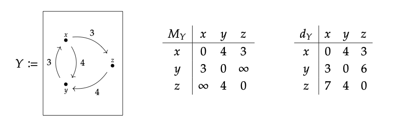
Here we fully explain how to compute dY using only MY. The matrix MY can be thought of as recording the length of paths that traverse either 0 or 1 edges: the diagonals being 0 mean we can get from x to x without traversing any edges. When we can get from x to y in one edge we record its length in MY , otherwise we use ∞.

When we multiply \(M_{Y}\) by itself using the formula Eq. (2.101), the result \(M_{Y}^{2}\) tells us the length of the shortest path traversing 2 edges or fewer. Similarly \(M_{Y}^{3}\) tells us about the shortest path traversing 3 edges or fewer:

One sees that the powers stabilize: \(M_{Y}^{2}\) = \(M_{Y}^{3}\); as soon as that happens one has the matrix of distances, \(d_{Y}\). Indeed \(M_{Y}^{n}\) records the lengths of the shortest path traverse n edges or fewer, and the powers will always stabilize if the set of vertices is finite, since the shortest path from one vertex to another will never visit a given vertex more than once.\(^{7}\)

Exercise 2.105.

Recall from Exercise 2.60 the matrix \(M_{X}\), for X as in Eq. (2.56). Calculate \(M_{X}^{2}\), \(M_{X}^{3}\), and \(M_{X}^{4}\). Check that \(M_{X}^{4}\) is what you got for the distance matrix in Exercise 2.58. ♦

This procedure gives an algorithm for computing the V-category presented by any V-weighted graph using matrix multiplication.