3.1: What is a Database?

Integrating data from disparate sources is a major problem in industry today. A study in 2008 [BH08] showed that data integration accounts for 40% of IT (information technology) budgets, and that the market for data integration software was $2.5 billion in 2007 and increasing at a rate of more than 8% per year. In other words, it is a major problem; but what is it?

A database is a system of interlocking tables. Data becomes information when it is stored in a given formation. That is, the numbers and letters don’t mean anything until they are organized, often into a system of interlocking tables. An organized system of interlocking tables is called a database. Here is a favorite example:

(3.1) These two tables interlock by use of a special left-hand column, demarcated by a vertical line; it is called the ID column. The ID column of the first table is called ‘Employee,’ and the ID column of the second table is called ‘Department.’ The entries in the ID column—e.g. 1, 2, 3 or 101, 102—are like row labels; they indicate a whole row of the table they’re in. Thus each row label must be unique (no two rows in a table can have the same label), so that it can unambiguously specify its row.

Each table’s ID column, and the set of unique identifiers found therein, is what allows for the interlocking mentioned above. Indeed, other entries in various tables can reference rows in a given table by use of its ID column. For example, each entry in the WorksIn column references a department for each employee; each entry in the Mngr (manager) column references an employee for each employee, and each entry in the Secr (secretary) column references an employee for each department. Managing all this cross-referencing is the purpose of databases.

Looking back at Eq. (3.1), one might notice that every non-ID column, found in either table, is a reference to a label of some sort. Some of these, namely WorksIn, Mngr, and Secr, are internal references, often called foreign keys; they refer to rows (keys) in the ID column of some (foreign) table. Others, namely FName and DName, are external references; they refer to strings or integers, which can also be thought of as labels, whose meaning is known more broadly. Internal reference labels can be changed as long as the change is consistent—1 could be replaced by 1001 everywhere without changing the meaning—whereas external reference labels certainly cannot! Changing Ruth to Bruce everywhere would change how people understood the data.

The reference structure for a given database—i.e. how tables interlock via foreign keys—tells us something about what information was intended to be stored in it. One may visualize the reference structure for Eq. (3.1) graphically as follows:

This is a kind of “Hasse diagram for a database,” much like the Hasse diagrams for preorders in Remark 1.39. How should you read it?

The two tables from Eq. (3.1) are represented in the graph (3.2) by the two black nodes, which are given the same name as the ID columns: Employee and Department. There is another node—drawn white rather than black—which represents the external reference type of strings, like “Alan,” “Alpha,” and “Sales". The arrows in the diagram represent non-ID columns of the tables; they point in the direction of reference: WorksIn refers an employee to a department.

Exercise 3.3.

Count the number of non-ID columns in Eq. (3.1). Count the number of arrows (foreign keys) in Eq. (3.2). They should be the same number in this case; is this a coincidence? ♦

A Hasse-style diagram like the one in Eq. (3.2) can be called a database schema; it represents how the information is being organized, the formation in which the data is kept. One may add rules, sometimes called ‘business rules’ to the schema, in order to ensure the integrity of the data. If these rules are violated, one knows that data being entered does not conform to the way the database designers intended. For example, the designers may enforce rules saying

• every department’s secretary must work in that department;

• every employee’s manager must work in the same department as the employee.

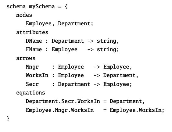
Doing so changes the schema, say from ‘easySchema’ (3.2) to ‘mySchema’ below.

In other words, the difference is that easySchema plus constraints equals mySchema. We will soon see that database schemas are categories C, that the data itself is given by a ‘set-valued’ functor C → Set, and that databases can be mapped to each other via functors C → D. In other words, there is a relatively large overlap between database theory and category theory. This has been worked out in a number of papers; see Section 3.6. It has also been implemented in working software, called FQL, which stands for functorial query language. Here is example FQL code for the schema shown above:

Communication between databases. We have said that databases are designed to store information about something. But different people or organizations might view the same sort of thing in different ways. For example, one bank stores its financial records according to European standards and another does so according to Japanese standards. If these two banks merge into one, they will need to be able to share their data despite differences in the shape of their database schemas.

Such problems are huge and intricate in general, because databases often comprise hundreds or thousands of interlocking tables. Moreover, these problems occur more frequently than just when companies want to merge. It is quite common that a given company moves data between databases on a daily basis. The reason is that different ways of organizing information are convenient for different purposes. Just like we pack our clothes in a suitcase when traveling but use a closet at home, there is generally not one best way to organize anything.

Category theory provides a mathematical approach for translating between these different organizational forms. That is, it formalizes a sort of automated reorganizing process called data migration, which takes data that fits snugly in one schema and moves it into another.

Here is a simple case. Imagine an airline company has two different databases, perhaps created at different times, that hold roughly the same data.

Schema A has more detail than schema B—an airline seat may be in first class or economy—but they are roughly the same. We will see that they can be connected by a functor, and that data conforming to A can be migrated through this functor to schema B and vice versa.

The statistics at the beginning of this section show that this sort of problem— when occurring at enterprise scale—continues to prove difficult and expensive. If one attempts to move data from a source schema to a target schema, the migrated data could fail to fit into the target schema or fail to satisfy some of its constraints. This happens surprisingly often in the world of business: a night may be spent moving data, and the next morning it is found to have arrived broken and unsuitable for further use. In fact, it is believed that over half of database migration projects fail.

In this chapter, we will discuss a category-theoretic method for migrating data. Using categories and functors, one can prove up front that a given data migration will not fail, i.e. that the result is guaranteed to fit into the target schema and satisfy all its constraints.

The material in this chapter gets to the heart of category theory: in particular, we discuss categories, functors, natural transformations, adjunctions, limits, and colimits. In fact, many of these ideas have been present in the discussion above:

• The schema pictures, e.g. Eq. (3.4) depict categories C.

• The instances, e.g. Eq. (3.1) are functors from C to a certain category called Set.

• The implicit mapping in Eq. (3.5), which takes economy and first class seats in A to airline seats in B, constitutes a functor A → B.

• The notion of data migration for moving data between schemas is formalized by adjoint functors.

We begin in Section 3.2 with the definition of categories and a bunch of different

sorts of examples. In Section 3.3 we bring back databases, in particular their instances and the maps between them, by discussing functors and natural transformations. In Section 3.4 we discuss data migration by way of adjunctions, which generalize the Galois connections we introduced in Section 1.4. Finally in Section 3.5 we give a bonus section on limits and colimits.\(^{1}\)