3.3: Functors, natural transformations, and databases

In Section 3.1 we showed some database schemas: graphs with path equations. Then in Section 3.2.2 we said that graphs with path equations correspond to finitely-presented categories. Now we want to explain what the data in a database is, as a way to introduce functors. To do so, we begin by noticing that sets and functions the objects and morphisms in the category Set can be captured by particularly simple databases.

Sets and functions as databases

The first observation is that any set can be understood as a table with only one column: the ID column.

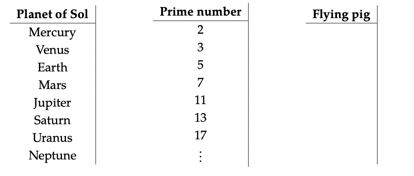
Rather than put the elements of the set between braces, e.g. {2, 3, 5, 7, 11, . . .}, we write them down as rows in a table.

In databases, single-column tables are often called controlled vocabularies, or master data. Now to be honest, we can only write out every single entry in a table when its set of rows is finite. A database practitioner might find the idea of our prime number table a bit unrealistic. But we’re mathematicians, so since the idea makes perfect sense abstractly, we will continue to think of sets as one-column tables.

The above databases have schemas consisting of just one vertex:

Obviously, there’s really not much difference between these schemas, other than the label of the unique vertex. So we could say “sets are databases whose schema consists of a single vertex.” Let’s move on to functions.

A function f : A → B can almost be depicted as a two-column table

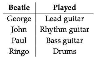
except it is unclear whether the elements of the right-hand column exhaust all of B. What if there are rock-and-roll instruments out there that none of the Beatles played? So a function f : A → B requires two tables, one for A and its f column, and one for B:

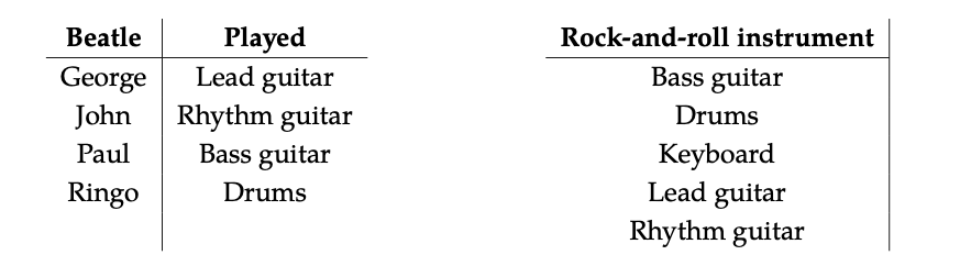
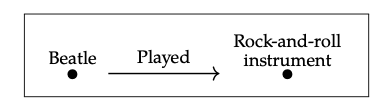
Thus the database schema for any function is just a labeled version of 2:

The lesson is that an instance of a database takes a presentation of a category, and turns every vertex into a set, and every arrow into a function. As such, it describes a map from the presented category to the category Set. In Section 2.4.2 we saw that maps ofV-categories are known as V-functors. Similarly, we call maps of plain old categories, functors.

Functors

A functor is a mapping between categories. It sends objects to objects and morphisms to morphisms, all while preserving identities and composition. Here is the formal definition.

Definition: 3.3.5.

Let C and D be categories. To specify a functor from C to D, denoted F : C → D,

(i) for every object c \(\in\) Ob(C), one specifies an object F(c) \(\in\) Ob(D);

(ii) for every morphism f : c1 → c2 in C, one specifies a morphism F(f ): F(\(c_{1}\)) → F(\(c_{2}\)) in D.

The above constituents must satisfy two properties:

(a) for every object c \(\in\) Ob(C), we have F(\(id_{c}\)) = \(id_{F(c)}\).
(b) for every three objects \(c_{1}\), \(c_{2}\), \(c_{3}\) \(\in\) Ob(C) and two morphisms f \(\in\) C(c1, c2), g \(\in\) C(\(c_{2}\),\(c_{3}\)), the equation F(f ; g) = F(f ) ; F(f ; g) holds in D.

Example 3.36.

For example, here we draw three functors F : 2 → 3:

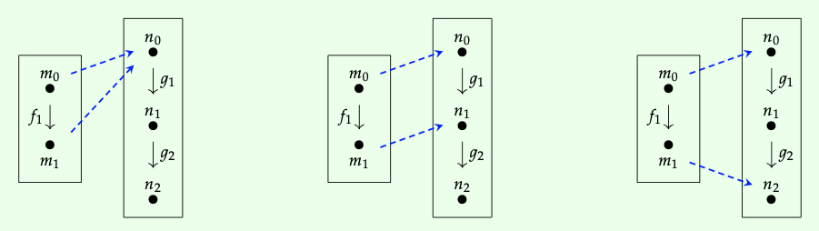
In each case, the dotted arrows show what the functor F does to the vertices in 2; once that information is specified, it turns out in this special case that what F does to the three paths in 2 is completely determined. In the left-hand diagram, F sends every path to the trivial path, i.e. the identity on \(n_{0}\). In the middle diagram F(\(m_{0}\)) = \(n_{0}\), F(\(f_{1}\)) = \(g_{1}\), and F(\(m_{1}\)) = \(n_{1}\). In the right-hand diagram, F(\(m_{0}\)) = \(n_{0}\), F(\(m_{1}\)) = \(n_{2}\), and F(\(f_{1}\)) = \(g_{1}\) ; \(g_{2}\).

Exercise 3.37.

Above we wrote down three functors 2 → 3. Find and write down all the remaining functors 2 → 3 ♦

Example 3.38.

Recall the categories presented by Free_square and Comm_square in Section 3.2.2. Here they are again, with' added to the labels in Free_square to help distinguish them:

There are lots of functors from the free square category (let’s call it F) to the commutative square category (let’s call it C).

However, there is exactly one functor F : F → C that sends A′ to A, B′ to B, C′ to C, and D′ to D. That is, once we have made this decision about how F acts on objects, each of the ten paths in F is forced to go to a certain path in C: the one with the right source and target.

Exercise 3.39.

Say where each of the ten morphisms in F is sent under the functor F from Example 3.38. ♦

All of our example functors so far have been completely determined by what they do on objects, but this is usually not the case.

Exercise 3.40.

Consider the free categories \(\mathcal{C}=\bullet \rightarrow \bullet \text { and } \mathcal{D}=\bullet \rightrightarrows \bullet\).

Give two functors F, G : C → D that act the same on objects but differently on morphisms. ♦

Example 3.41.

There are also lots of functors from the commutative square category C to the free square category F, but none that sends A to A′, B to B′, C to C′, and D to D′. The reason is that if F were such a functor,then since f ; h = g ; i in C, we would have F(f ; h) = F(g ; i), but then the rules of functors would let us reason as follows:

The resulting equation, f' ; h' = g' ; i' does not hold in F because it is a free category (there are “no equations”): every two paths are considered different morphisms. Thus our proposed F is not a functor.

Example 3.42 (Functions between preorders are montone maps).

Recall from Section 3.2.3 that preorders are categories with at most one morphism between any two objects. A functor between preorders is exactly a monotone map.

For example, consider the preorder (\(\mathbb{N}\), ≤) considered as a category N with objects Ob(N) = \(\mathbb{N}\) and a unique morphism m → n iff m ≤ n. A functor F : N → N sends each object n \(\in\) \(\mathbb{N}\) to an object F(n) \(\in\) \(\mathbb{N}\). It must send morphisms in N to morphisms in \(\mathbb{N}\). This means if there is a morphism m → n then there had better be a morphism F(m) → F(n). In other words, if m ≤ n, then we had better have F(m) ≤ F(n). But as long as m ≤ n implies F(m) ≤ F(n), we have a functor.

Thus a functor F : N → N and a monotone map \(\mathbb{N}\) → \(\mathbb{N}\) are the same thing.

Exercise 3.43 (The category of categories).

Back in the primordial ooze, there is a category Cat in which the objects are themselves categories. Your task here is to construct this category.

1. Given any category C, show that there exists a functor \(id_{C}\) : C → C, known as the identity functor on C, that maps each object to itself and each morphism to itself.

Note that a functor C → D consists of a function from Ob(C) to Ob(D) and for each pair of objects \(c_{1}\), \(c_{2}\) \(\in\) C a function from C(\(c_{1}\), \(c_{2}\)) to D(\(c_{1}\), \(c_{2}\)).

2. Show that given F: C → D and G: D → E, we can define a new functor (F ; G): C → E just by composing functions.

3. Show that there is a category, call it Cat, where the objects are categories, mor- phisms are functors, and identities and composition are given as above. ♦

Database instances as Set-valued functors

Let C be a category, and recall the category Set from Definition 3.24. Set is known as a set-valued functor on C. Much of database theory (not how to make them fast, but what they are and what you do with them) can be cast in this light. A functor F : C → Set is known as a set-valued functor on C. Indeed, we already saw in Remark 3.20 that any database schema can be regarded as (presenting) a category C. The next thing to notice is that the data itself any instance of the database is given by a set-valued functor I : C → Set. The only additional string detail is that for any white node, such as \(c=\stackrel{\text { string }}{\circ}\), we want to force I to map to the set of strings. We suppress this detail in the following definition.

Definition: 3.44.

Let C be a schema, i.e. a finitely-presented category. A C-instance is a functor I : C → Set.\(^{5}\)

Exercise 3.45.

Let 1 denote the category with one object, called 1, one identity morphism \(id_{1}\), and no other morphisms. For any functor F: 1 → Set one can extract a set F(1). Show that for any set S, there is a functor \(F_{S}\) : 1 → Set such that \(F_{S}\)(1) = S. ♦

The above exercise reaffirms that the set of planets, the set of prime numbers, and the set of flying pigs are all set-valued functors instances on the schema 1. Similarly, set-valued functors on the category 2 are functions. All our examples so far are for the situation where the schema is a free category (no equations). Let’s try an example of a category that is not free.

Example 3.46.

Consider the following category:

What is a set-valued functor F : C → Set? It will consist of a set Z := F(z) and a function S := F(s): Z → Z, subject to the requirement that S ; S = S. Here are some examples

• Z is the set of US citizens, and S sends each citizen to her or his president. The president’s president is her or him-self.

• Z = \(\mathbb{N}\) is the set of natural numbers and S sends each number to 0. In particular, 0 goes to itself.

• Z is the set of all well-formed arithmetic expressions, such as 13 + (2 ∗ 4) or −5, that one can write using integers and the symbols +, −, ∗, (,). The function S evaluates the expression to return an integer, which is itself a well-formed expression. The evaluation of an integer is itself.

• Z = \(\mathbb{N}\) \(_{≥2}\), and S sends n to its smallest prime factor. The smallest prime factor of a prime is itself.

Exercise 3.48.

Above, we thought of the sort of data that would make sense for the schema (3.47). Give an example of the sort of data that would make sense for the following schemas:

The main idea is this: a database schema is a category, and an instance on that schema the data itself is a set-valued functor. All the constraints, or business rules, are ensured by the rules of functors, namely that functors preserve composition.\(^{6}\)

Natural transformations

If C is a schema i.e. a finitely-presented category then there are many database instances on it, which we can organize into a category. But this is part of a larger story, namely that of natural transformations. An abstract picture to have in mind is this:

Definition: 3.49.

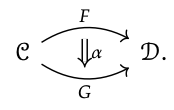
Let C and D be categories, and let F, G : C → D be functors. To specify a natural transformation α : F ⇒ G,

(i) for each object c \(\in\) C, one specifies a morphism \(α_{c}\) : F(c) → G(c) in D, called the c-component of α.

These components must satisfy the following, called the naturality condition:

(a) for every morphism f : c → d in C, the following equation must hold:

F( f ) ; \(α_{d}\) = \(α_{c}\) ; G( f ).

A natural transformation α : F → G is called a natural isomorphism if each component \(α_{c}\) is an isomorphism in D.

The naturality condition can also be written as a so-called commutative diagram. A diagram in a category is drawn as a graph whose vertices and arrows are labeled by objects and morphisms in the category. For example, here is a diagram that’s relevant to the naturality condition in Definition 3.49:

Definition: 3.51.

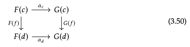
A diagram D in C is a functor D : J → C from any category J, called the indexing category of the diagram D. We say that D commutes if D( f ) = D( f ′) holds for every parallel pair of morphisms f, f′: a → b in J.\(^{7}\)

In terms of Eq. (3.50), the only case of two parallel morphisms is that of F(c) ⇒ G(d), so to say that the diagram commutes is to say that F(f) ; \(α_{d}\) = \(α_{c}\) ; G(f).Thisisexactly the naturality condition from Definition 3.49.

Example 3.52.

A representative picture is as follows:

We have depicted, in blue and red respectively, two functors F, G : C → D. A natural transformation α: F ⇒ G is given by choosing components \(α_{1}\) : v → x and \(α_{2}\) : w → y. We have highlighted the only choice for each in green; namely, \(α_{1}\) = c and \(α_{2}\) = g.

The key point is that the functors F and G are ways of viewing the category C as lying inside the category D. The natural transformation α, then, is a way of relating these two views using the morphisms in D. Does this help you to see and appreciate the notation

Example 3.53.

We said in Exercise 3.45 that a functor 1 → Set can be identified with a set. So suppose A and B are sets considered as functors A, B : 1 → Set. A natural transformation between these functors is just a function between the sets.

Definition: 3.54.

Let C and D be categories. We denote by \(D^{C}\) the category whose objects are functors F : C → D and whose morphisms \(D^{C}\)(F, G) are the natural transformations α : F → G. This category \(D^{C}\) is called the functor category, or the category of functors from C to D.

Exercise 3.55.

Let’s look more deeply at how \(D^{C}\) is a category.

1. Figure out how to compose natural transformations. (Hint: an expert tells you “for each object c \(\in\) C, compose the c-components.”)
2. Propose an identity natural transformation on any object F \(\in\) \(D^{C}\), and check that it is unital (i.e. that it obeys condition (a) of Definition 3.6). ♦

Example 3.56.

In our new language, Example 3.53 says that \(Set^{1}\) is equivalent to Set.

Example 3.57.

Let N denote the category associated to the preorder (\(\mathbb{N}\), ≤), and recall from Example 3.42 that we can identify a functor F : N → N with a non-decreasing sequence (\(F_{0}\), \(F_{1}\), \(F_{2}\),...) of natural numbers, i.e. \(F_{0}\) ≤ \(F_{1}\) ≤ \(F_{2}\) ≤ ···. If G is another functor, considered as a non-decreasing sequence, then what is a natural transformation α: F → G? Since there is at most one morphism between two objects in a preorder, each component \(a_{n}\) : \(F_{n}\) → \(G_{n}\) has no data, it just tells us a fact: that \(F_{n}\) ≤ \(G_{n}\). And the naturality condition is vacuous: every square in a preorder commutes. So a natural transforma- tion between F and G exists iff \(F_{n}\) ≤ \(G_{n}\) for each n, and any two natural transformations F ⇒ G are the same. In other words, the category \(N^{N}\) is itself a preorder; namely the preorder of monotone maps \(\mathbb{N}\) → \(\mathbb{N}\).

Exercise 3.58.

Let C be an arbitrary category and let P be a preorder, thought of as a category. Consider the following statements:

1. For any two functors F, G : C → P, there is at most one natural transformation F → G.

2. For any two functors F, G : P → C, there is at most one natural transformation F → G.

For each, if it is true, say why; if it is false, give a counterexample. ♦

Remark 3.59. Recall that in Remark 2.71 we said the category of preorders is equivalent to the category of Bool-categories. We can now state the precise meaning of this sentence. First, there exists a category PrO in which the objects are preorders and the morphisms are monotone maps. Second, there exists a category Bool-Cat in which the objects are Bool-categories and the morphisms are Bool-functors. We call these two categories equivalent because there exist functors F : PrO → Bool-Cat and G : Bool-Cat → PrO such that there exist natural isomorphisms F ; G \(\cong\) \(id_{PrO}\) and G ; F \(\cong\) \(id_{Bool-Cat}\) in the sense of Definition 3.49.

The category of instances on a schema

Definition: 3.60.

Suppose that C is a database schema and I , J : C → Set are database instances. An instance homomorphism between them is a natural transformation α : I → J. Write C-Inst := \(Set^{C}\) to denote the functor category as defined in Definition 3.54.

We saw in Example 3.53 that 1-Inst is equivalent to the category Set. In this subsection, we will show that there is a schema whose instances are graphs and whose instance homomorphisms are graph homomorphisms.

Extended example: the category of graphs as a functor category. You may find yourself back in the primordial ooze (first discussed in Section 2.3.2), because while previously we have been using graphs to present categories, now we obtain graphs themselves as database instances on a specific schema (which is itself a graph):

Here’s an example Gr-instance, i.e. set-valued functor I : Gr → Set, in table form:

Here I(Arrow) = {a, b, c, d, e}, and I(Vertex) = {1, 2, 3, 4}. One can draw the instance I as a graph:

Every row in the Vertex table is drawn as a vertex, and every row in the Arrow table is drawn as an arrow, connecting its specified source and target. Every possible graph can be written as a database instance on the schema Gr, and every possible Gr-instance can be represented as a graph.

Exercise 3.62.

In Eq. (3.2), a graph is shown (forget the distinction between white and black nodes). Write down the corresponding Gr-instance, as in Eq. (3.61). (Do not be concerned that you are in the primordial ooze. ♦

Thus the objects in the category Gr-Inst are graphs. The morphisms in Gr-Inst are called graph homomorphisms. Let’s unwind this. Suppose that G, H : Gr → Set are functors (i.e. Gr-instances); that is, they are objects G, H \(\in\) Gr-Inst. A morphism G → H is a natural transformation α : G → H between them; what does that entail?

By Definition 3.49, since Gr has two objects, α consists of two components,

\(α_{Vertex}\) : G(Vertex) → H(Vertex) and \(α_{Arrow}\) : G(Arrow) → H(Arrow),

both of which are morphisms in Set. In other words, α consists of a function from vertices of G to vertices of H and a function from arrows of G to arrows of H. For these functions to constitute a graph homomorphism, they must “respect source and target” in the precise sense that the naturality condition, Eq. (3.50) holds. That is, for every morphism in Gr, namely source and target, the following diagrams must commute:

These may look complicated, but they say exactly what we want. We want the functions \(α_{Vertex}\) and \(α_{Arrow}\) to respect source and targets in G and H. The left diagram says “start with an arrow in G. You can either apply α to the arrow and then take its source in H, or you can take its source in G and then apply α to that vertex; either way you get the same answer.” The right-hand diagram says the same thing about targets.

Example 3.63.

Consider the graphs G and H shown below

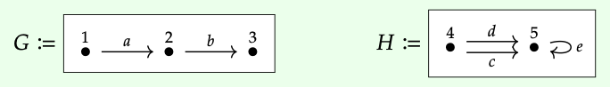
Here they are, written as database instances—i.e. set-valued functors—on Gr:

The top row is G and the bottom row is H. They are offset so you can more easily complete the following exercise.

Exercise 3.64.

We claim that with G, H as in Example 3.63 there is exactly one graph homomorphism α : G → H such that \(α_{Arrow}\)(a) = d.

1. What is the other value of \(α_{Arrow}\), and what are the three values of \(α_{Vertex}\)?

2. In your own copy of the tables of Example 3.63, draw \(α_{Arrow}\) as two lines connecting the cells in the ID column of G(Arrow) to those in the ID column of H(Arrow). Similarly, draw \(α_{Vertex}\) as connecting lines.

3. Check the source column and target column and make sure that the matches are natural, i.e. that “alpha then source equals source then alpha” and similarly for “target.” ♦