2.4: Fluid mechanics- Drag

The preceding examples showed that easy cases can check and construct formulas, but the examples can be done without easy cases (for example, with calculus). For the next equations, from fluid mechanics, no exact solutions are known in general, so easy cases and other street-fighting tools are almost the only way to make progress.

Here then are the Navier–Stokes equations of fluid mechanics:

\[\frac{\partial \mathbf{v}}{\partial t}+(\mathbf{v} \cdot \boldsymbol{\nabla}) \mathbf{v}=-\frac{1}{\rho} \boldsymbol{\nabla} p+v \boldsymbol{\nabla}^{2} \mathbf{v}\label{2.13} \]

where v is the velocity of the fluid (as a function of position and time), \(ρ\) is its density, \(p\) is the pressure, and \(ν\) is the kinematic viscosity. These equations describe an amazing variety of phenomena including flight, tornadoes, and river rapids.

Our example is the following home experiment on drag. Photocopy this page while magnifying it by a factor of 2; then cut out the following two templates:

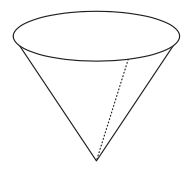
With each template, tape together the shaded areas to make a cone. The two resulting cones have the same shape, but the large cone has twice the height and width of the small cone.

Question

When the cones are dropped point downward, what is the approximate ratio of their terminal speeds (the speeds at which drag balances weight)?

The Navier–Stokes equations contain the answer to this question. Finding the terminal speed involves four steps.

Step 1. Impose boundary conditions. The conditions include the motion of the cone and the requirement that no fluid enters the paper.

Step 2. Solve the equations, together with the continuity equation \(∇·v = 0\), in order to find the pressure and velocity at the surface of the cone.

Step 3. Use the pressure and velocity to find the pressure and velocity gradient at the surface of the cone; then integrate the resulting forces to find the net force and torque on the cone.

Step 4. Use the net force and torque to find the motion of the cone. This step is difficult because the resulting motion must be consistent with the motion assumed in step 1. If it is not consistent, go back to step 1, assume a different motion, and hope for better luck upon reaching this step.

Unfortunately, the Navier–Stokes equations are coupled and nonlinear partial-differential equations. Their solutions are known only in very simple cases: for example, a sphere moving very slowly in a viscous fluid, or a sphere moving at any speed in a zero-viscosity fluid. There is little hope of solving for the complicated flow around an irregular, quivering shape such as a flexible paper cone.

Multiple Problems

Problem 2.12 Checking dimensions in the Navier–Stokes equations

Check that the first three terms of the Navier–Stokes equations have identical dimensions.

Problem 2.13 Dimensions of kinematic viscosity

From the Navier–Stokes equations, find the dimensions of kinematic viscosity \(ν\).

Using dimensions

Because a direct solution of the Navier–Stokes equations is out of the question, let’s use the methods of dimensional analysis and easy cases. A direct approach is to use them to deduce the terminal velocity itself. An indirect approach is to deduce the drag force as a function of fall speed and then to find the speed at which the drag balances the weight of the cones. This two-step approach simplifies the problem. It introduces only one new quantity (the drag force) but eliminates two quantities: the gravitational acceleration and the mass of the cone.

Problem 2.14 Explaining the simplification

Why is the drag force independent of the gravitational acceleration \(g\) and of the cone’s mass \(m\) (yet the force depends on the cone’s shape and size)?

The principle of dimensions is that all terms in a valid equation have identical dimensions.

Applied to the drag force \(F\), it means that in the equation \(F = f\)(quantities that affect F) both sides have dimensions of force. Therefore, the strategy is to find the quantities that affect \(F\), find their dimensions, and then combine the quantities into a quantity with dimensions of force.

Question

On what quantities does the drag depend, and what are their dimensions?

The drag force depends on four quantities: two parameters of the cone and two parameters of the fluid (air). (For the dimensions of ν, see Problem 2.13.)

V	speed of the cone	LT\(^{-1}\)
r	size of the cone	L
p	density of the air	ML\(^{-3}\)
v	viscosity of the air	L\(^{2}\)T\(^{-1}\)

Question

Do any combinations of the four parameters \(v\), \(r\), \(ρ\), and \(ν\) have dimensions of force?

The next step is to combine \(v\), \(r\), \(ρ\), and \(ν\) into a quantity with dimensions of force. Unfortunately, the possibilities are numerous for example,

\[F_{1} = ρv^{2}r^{2}, F_{2} = ρνvr, \label{2.14} \]

or the product combinations \(\sqrt{F_{1}F_{2}} \text{ and } F_{1}^{2}/F_{2}\). Any sum of these ugly \(1 \sqrt{2}\) products is also a force, so the drag force \(F\) could be \(\sqrt{F1F2}\) + \(F_{1}^{2}/F_{2}\), 3\(\sqrt{F1F2} − 2F_{1}^{2}/F_{2}\), or much worse.

Narrowing the possibilities requires a method more sophisticated than simply guessing combinations with correct dimensions. To develop the sophisticated approach, return to the first principle of dimensions: All terms in an equation have identical dimensions. This principle applies to any statement about drag such as

\[A + B = C \label{2.15} \]

where the blobs \(A, B, \text{ and } C\) are functions of \(F, v, r, ρ, \text{ and } ν\). Although the blobs can be absurdly complex functions, they have identical dimensions. Therefore, dividing each term by \(A\), which produces the equation

\[\frac{A}{A} + \frac{B}{A} = \frac{C}{A}, \label{2.16} \]

makes each term dimensionless. The same method turns any valid equation into a dimensionless equation. Thus, any (true) equation describing the world can be written in a dimensionless form.

Any dimensionless form can be built from dimensionless groups: from dimensionless products of the variables. Because any equation describing the world can be written in a dimensionless form, and any dimensionless form can be written using dimensionless groups, any equation describing the world can be written using dimensionless groups.

Question

Is the free-fall example (Section 1.2) consistent with this principle?

Before applying this principle to the complicated problem of drag, try it in the simple example of free fall (Section 1.2). The exact impact speed of an object dropped from a height h is \(v = \sqrt{2gh}\), where g is the gravitational acceleration. This result can indeed be written in the dimensionless form \(v/\sqrt{gh}\) = \(\sqrt{2}\), which itself uses only the dimensionless group \(v/\sqrt{gh}\). The new principle passes its first test.

This dimensionless-group analysis of formulas, when reversed, becomes a method of synthesis. Let’s warm up by synthesizing the impact speed v. First, list the quantities in the problem; here, they are v, g, and h. Second, combine these quantities into dimensionless groups. Here, all dimensionless groups can be constructed just from one group. For that group, let’s choose \(v^{2}/gh\) (the particular choice does not affect the conclusion). Then the only possible dimensionless statement is

\[\frac{v^{2}}{gh} = \text{ dimensionless constant }\label{2.17} \]

(The right side is a dimensionless constant because no second group is available to use there.) In other words, \(v^{2}/gh ∼ 1\) or \(v ∼ \sqrt{gh}\).

This result reproduces the result of the less sophisticated dimensional analysis in Section 1.2. Indeed, with only one dimensionless group, either analysis leads to the same conclusion. However, in hard problems for example, finding the drag force the less sophisticated method does not provide its constraint in a useful form; then the method of dimensionless groups is essential.

Multiple Problems

Problem 2.15 Fall time

Synthesize an approximate formula for the free-fall time \(t \text{ from } g \text{ and } h\).

Problem 2.16 Kepler’s third law

Synthesize Kepler’s third law connecting the orbital period of a planet to its orbital radius. (See also Problem 1.15.)

Question

What dimensionless groups can be constructed for the drag problem?

One dimensionless group could be \(F/ρv^{2}r^{2}\); a second group could be rv/ν. Any other group can be constructed from these groups (Problem 2.17), so the problem is described by two independent dimensionless groups. The most general dimensionless statement is then

\[\text{ one group = f(second group) }, \label{2.18} \]

where \(f\) is a still-unknown (but dimensionless) function.

Question

Which dimensionless group belongs on the left side?

The goal is to synthesize a formula for \(F, \text{ and } F\) appears only in the first group \(F/ρv^{2}r^{2}\). With that constraint in mind, place the first group on the left side rather than wrapping it in the still-mysterious function \(f\). With this choice, the most general statement about drag force is

\[\frac{F}{pv^{2}r^{2}} = f\frac{rv}{v}. \label{2.19} \]

The physics of the (steady-state) drag force on the cone is all contained in the dimensionless function \(f\).

Multiple problems

Problem 2.17 Only two groups

Show that \(F, v, r, ρ, \text{ and } ν\) produce only two independent dimensionless groups.

Problem 2.18 How many groups in general?

Is there a general method to predict the number of independent dimensionless groups? (The answer was given in 1914 by Buckingham [9].)

The procedure might seem pointless, having produced a drag force that depends on the unknown function f. But it has greatly improved our chances of finding \(f\). The original problem formulation required guessing the four-variable function h in \(F = h(v, r, ρ, ν)\), whereas dimensional analysis reduced the problem to guessing a function of only one variable (the ratio \(vr/ν\)). The value of this simplification was eloquently described by the statistician and physicist Harold Jeffreys (quoted in [34, p. 82]):

A good table of functions of one variable may require a page; that of a function of two variables a volume; that of a function of three variables a bookcase; and that of a function of four variables a library.

Problem 2.19 Dimensionless groups for the truncated pyramid

The truncated pyramid of Section 2.3 has volume

\[V = \frac{1}{3}h (a^{2} + ab + b^{2}). \label{2.20} \]

Make dimensionless groups from \(V, h, a, \text{ and } b\), and rewrite the volume using these groups. (There are many ways to do so.)

Using easy cases

Although improved, our chances do not look high: Even the one-variable drag problem has no exact solution. But it might have exact solutions in its easy cases. Because the easiest cases are often extreme cases, look first at the extreme cases.

Question

Extreme cases of what?

The unknown function \(f\) depends on only \(rv/ν\),

\[\frac{F}{pv^{2}r^{2}} = f \frac{rv}{v}, \label{2.21} \]

so try extremes of \(rv/ν\). However, to avoid lapsing into mindless symbol pushing, first determine the meaning of \(rv/ν\). This combination \(rv/ν\), often denoted Re, is the famous Reynolds number. (Its physical interpretation requires the technique of lumping and is explained in Section 3.4.3.) The Reynolds number affects the drag force via the unknown function \(f\):

\[\frac{F}{pv^{2}r^{2}} = f(Re). \label{2.22} \]

With luck, \(f\) can be deduced at extremes of the Reynolds number; with further luck, the falling cones are an example of one extreme.

Question

Are the falling cones an extreme of the Reynolds number?

The Reynolds number depends on \(r, v, \text{ and } ν\). For the speed v, everyday experience suggests that the cones fall at roughly 1 m\(s^{-1}\) (within, say, a factor of 2). The size \(r\) is roughly 0.1 m (again within a factor of 2). And the kinematic viscosity of air is \(ν ∼ 10^{-5}m^{2}s^{-1}\). The Reynolds number is

\[\frac{\overbrace{0.1 \mathrm{~m}}^{\mathrm{r}} \times \overbrace{1 \mathrm{~m} \mathrm{~s}^{-1}}^{v}}{\underbrace{10^{-5} \mathrm{~m}^{2} \mathrm{~s}^{-1}}_{\mathrm{v}}} \sim 10^{4}\label{2.23} \]

It is significantly greater than 1, so the falling cones are an extreme case of high Reynolds number. (For low Reynolds number, try Problem 2.27 and see [38].)

Problem 2.20 Reynolds numbers in everyday flows

Estimate Re for a submarine cruising underwater, a falling pollen grain, a falling raindrop, and a 747 crossing the Atlantic.

The high-Reynolds-number limit can be reached many ways. One way is to shrink the viscosity \(ν \text{ to } 0\), because ν lives in the denominator of the Reynolds number. Therefore, in the limit of high Reynolds number, viscosity disappears from the problem and the drag force should not depend on viscosity. This reasoning contains several subtle untruths, yet its conclusion is mostly correct. (Clarifying the subtleties required two centuries of progress in mathematics, culminating in singular perturbations and the theory of boundary layers [12, 46].)

Viscosity affects the drag force only through the Reynolds number:

\[\frac{F}{pv^{2}r^{2}} = f(\frac{rv}{v}). \label{2.34} \]

To make \(F\) independent of viscosity, \(F\) must be independent of Reynolds number! The problem then contains only one independent dimensionless group, \(F/ρv^{2}r^{2}\), so the most general statement about drag is

\[\frac{F}{pv^{2}r^{2}} = \text{ dimensional constant } \label{2.25} \]

The drag force itself is then \(F ∼ ρv^{2}r^{2}\). Because r is proportional to the cone’s cross-sectional area \(A\), the drag force is commonly written

\[F ∼ ρv^{2}A. \label{2.26} \]

Although the derivation was for falling cones, the result applies to any object as long as the Reynolds number is high. The shape affects only the missing dimensionless constant. For a sphere, it is roughly 1/4; for a long cylinder moving perpendicular to its axis, it is roughly 1/2; and for a flat plate moving perpendicular to its face, it is roughly

Terminal velocities

The result \(F ∼ ρv^{2}A\) is enough to predict the terminal velocities of the cones. Terminal velocity means zero acceleration, so the drag force must balance the weight. The weight is \(W = σ_{paper}A_{\text{paper}}g\), where \(σ_{\text{paper}}\) is the areal density of paper (mass per area) and \(A_{\text{paper}}\) is the area of the template after cutting out the quarter section. Because \(A_{\text{paper}}\) is comparable to the cross-sectional area \(A\), the weight is roughly given by

\[W ∼ σ_{\text{paper}}Ag. \label{2.27} \]

Therefore,

\[\underbrace{ρv^{2}A} \underbrace{∼ σ_{paper}Ag}.\label{2.28} \]

The area divides out and the terminal velocity becomes

\[v \sim \sqrt{\frac{g \sigma_{\text {paper }}}{\rho}} \label{2.29} \]

All cones constructed from the same paper and having the same shape, whatever their size, fall at the same speed!

To test this prediction, I constructed the small and large cones described on page 21, held one in each hand above my head, and let them fall. Their 2m fall lasted roughly 2s, and they landed within 0.1s of one another. Cheap experiment and cheap theory agree!

Multiple problems

Problem 2.21 Home experiment of a small versus a large cone

Try the cone home experiment yourself (page 21).

Problem 2.22 Home experiment of four stacked cones versus one cone

Predict the ratio

\[\frac{\text{ terminal velocity of four small cones stacked inside each other } }{ \text{ terminal velocity of one small cone }}. \label{2.30} \]

Test your prediction. Can you find a method not requiring timing equipment?

Problem 2.23 Estimating the terminal speed

Estimate or look up the areal density of paper; predict the cones’ terminal speed; and then compare that prediction to the result of the home experiment.