
3.2: The Definite Integral
- Page ID
- 71061

\( \newcommand{\vecs}[1]{\overset { \scriptstyle \rightharpoonup} {\mathbf{#1}} } \)
\( \newcommand{\vecd}[1]{\overset{-\!-\!\rightharpoonup}{\vphantom{a}\smash {#1}}} \)
\( \newcommand{\dsum}{\displaystyle\sum\limits} \)
\( \newcommand{\dint}{\displaystyle\int\limits} \)
\( \newcommand{\dlim}{\displaystyle\lim\limits} \)
\( \newcommand{\id}{\mathrm{id}}\) \( \newcommand{\Span}{\mathrm{span}}\)
( \newcommand{\kernel}{\mathrm{null}\,}\) \( \newcommand{\range}{\mathrm{range}\,}\)
\( \newcommand{\RealPart}{\mathrm{Re}}\) \( \newcommand{\ImaginaryPart}{\mathrm{Im}}\)
\( \newcommand{\Argument}{\mathrm{Arg}}\) \( \newcommand{\norm}[1]{\| #1 \|}\)
\( \newcommand{\inner}[2]{\langle #1, #2 \rangle}\)
\( \newcommand{\Span}{\mathrm{span}}\)
\( \newcommand{\id}{\mathrm{id}}\)
\( \newcommand{\Span}{\mathrm{span}}\)
\( \newcommand{\kernel}{\mathrm{null}\,}\)
\( \newcommand{\range}{\mathrm{range}\,}\)
\( \newcommand{\RealPart}{\mathrm{Re}}\)
\( \newcommand{\ImaginaryPart}{\mathrm{Im}}\)
\( \newcommand{\Argument}{\mathrm{Arg}}\)
\( \newcommand{\norm}[1]{\| #1 \|}\)
\( \newcommand{\inner}[2]{\langle #1, #2 \rangle}\)
\( \newcommand{\Span}{\mathrm{span}}\) \( \newcommand{\AA}{\unicode[.8,0]{x212B}}\)
\( \newcommand{\vectorA}[1]{\vec{#1}} % arrow\)
\( \newcommand{\vectorAt}[1]{\vec{\text{#1}}} % arrow\)
\( \newcommand{\vectorB}[1]{\overset { \scriptstyle \rightharpoonup} {\mathbf{#1}} } \)
\( \newcommand{\vectorC}[1]{\textbf{#1}} \)
\( \newcommand{\vectorD}[1]{\overrightarrow{#1}} \)
\( \newcommand{\vectorDt}[1]{\overrightarrow{\text{#1}}} \)
\( \newcommand{\vectE}[1]{\overset{-\!-\!\rightharpoonup}{\vphantom{a}\smash{\mathbf {#1}}}} \)
\( \newcommand{\vecs}[1]{\overset { \scriptstyle \rightharpoonup} {\mathbf{#1}} } \)
\(\newcommand{\longvect}{\overrightarrow}\)
\( \newcommand{\vecd}[1]{\overset{-\!-\!\rightharpoonup}{\vphantom{a}\smash {#1}}} \)
\(\newcommand{\avec}{\mathbf a}\) \(\newcommand{\bvec}{\mathbf b}\) \(\newcommand{\cvec}{\mathbf c}\) \(\newcommand{\dvec}{\mathbf d}\) \(\newcommand{\dtil}{\widetilde{\mathbf d}}\) \(\newcommand{\evec}{\mathbf e}\) \(\newcommand{\fvec}{\mathbf f}\) \(\newcommand{\nvec}{\mathbf n}\) \(\newcommand{\pvec}{\mathbf p}\) \(\newcommand{\qvec}{\mathbf q}\) \(\newcommand{\svec}{\mathbf s}\) \(\newcommand{\tvec}{\mathbf t}\) \(\newcommand{\uvec}{\mathbf u}\) \(\newcommand{\vvec}{\mathbf v}\) \(\newcommand{\wvec}{\mathbf w}\) \(\newcommand{\xvec}{\mathbf x}\) \(\newcommand{\yvec}{\mathbf y}\) \(\newcommand{\zvec}{\mathbf z}\) \(\newcommand{\rvec}{\mathbf r}\) \(\newcommand{\mvec}{\mathbf m}\) \(\newcommand{\zerovec}{\mathbf 0}\) \(\newcommand{\onevec}{\mathbf 1}\) \(\newcommand{\real}{\mathbb R}\) \(\newcommand{\twovec}[2]{\left[\begin{array}{r}#1 \\ #2 \end{array}\right]}\) \(\newcommand{\ctwovec}[2]{\left[\begin{array}{c}#1 \\ #2 \end{array}\right]}\) \(\newcommand{\threevec}[3]{\left[\begin{array}{r}#1 \\ #2 \\ #3 \end{array}\right]}\) \(\newcommand{\cthreevec}[3]{\left[\begin{array}{c}#1 \\ #2 \\ #3 \end{array}\right]}\) \(\newcommand{\fourvec}[4]{\left[\begin{array}{r}#1 \\ #2 \\ #3 \\ #4 \end{array}\right]}\) \(\newcommand{\cfourvec}[4]{\left[\begin{array}{c}#1 \\ #2 \\ #3 \\ #4 \end{array}\right]}\) \(\newcommand{\fivevec}[5]{\left[\begin{array}{r}#1 \\ #2 \\ #3 \\ #4 \\ #5 \\ \end{array}\right]}\) \(\newcommand{\cfivevec}[5]{\left[\begin{array}{c}#1 \\ #2 \\ #3 \\ #4 \\ #5 \\ \end{array}\right]}\) \(\newcommand{\mattwo}[4]{\left[\begin{array}{rr}#1 \amp #2 \\ #3 \amp #4 \\ \end{array}\right]}\) \(\newcommand{\laspan}[1]{\text{Span}\{#1\}}\) \(\newcommand{\bcal}{\cal B}\) \(\newcommand{\ccal}{\cal C}\) \(\newcommand{\scal}{\cal S}\) \(\newcommand{\wcal}{\cal W}\) \(\newcommand{\ecal}{\cal E}\) \(\newcommand{\coords}[2]{\left\{#1\right\}_{#2}}\) \(\newcommand{\gray}[1]{\color{gray}{#1}}\) \(\newcommand{\lgray}[1]{\color{lightgray}{#1}}\) \(\newcommand{\rank}{\operatorname{rank}}\) \(\newcommand{\row}{\text{Row}}\) \(\newcommand{\col}{\text{Col}}\) \(\renewcommand{\row}{\text{Row}}\) \(\newcommand{\nul}{\text{Nul}}\) \(\newcommand{\var}{\text{Var}}\) \(\newcommand{\corr}{\text{corr}}\) \(\newcommand{\len}[1]{\left|#1\right|}\) \(\newcommand{\bbar}{\overline{\bvec}}\) \(\newcommand{\bhat}{\widehat{\bvec}}\) \(\newcommand{\bperp}{\bvec^\perp}\) \(\newcommand{\xhat}{\widehat{\xvec}}\) \(\newcommand{\vhat}{\widehat{\vvec}}\) \(\newcommand{\uhat}{\widehat{\uvec}}\) \(\newcommand{\what}{\widehat{\wvec}}\) \(\newcommand{\Sighat}{\widehat{\Sigma}}\) \(\newcommand{\lt}{<}\) \(\newcommand{\gt}{>}\) \(\newcommand{\amp}{&}\) \(\definecolor{fillinmathshade}{gray}{0.9}\)Distance from Velocity
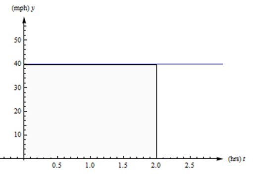
Suppose a car travels on a straight road at a constant speed of 40 miles per hour for two hours. See the graph of its velocity below. How far has it gone?
Solution
We all remember distance = rate\( \cdot \)time, so this one is easy. The car has gone (40 miles/hour)\( \cdot \)(2 hours) = 80 miles.
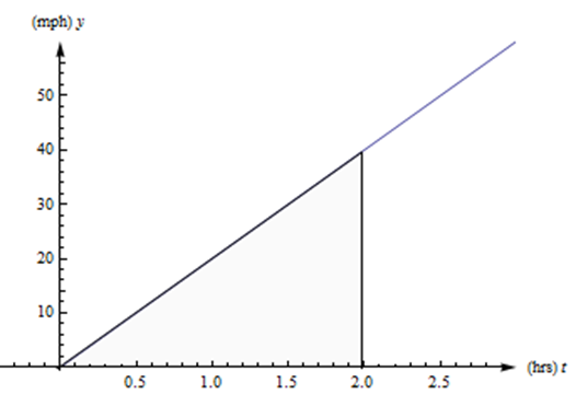
Now suppose that a car travels so that its speed increases steadily from 0 to 40 miles per hour, for two hours. (Just be grateful you weren’t stuck behind this car on the highway.) See the graph of its velocity in below. How far has this car gone?
Solution
The trouble with our old reliable distance = rate\( \cdot \)time relationship is that it only works if the rate is constant. If the rate is changing, there isn’t a good way to use this formula.
But look at the graph from the last example again. Notice that distance = rate\( \cdot \)time also describes the area between the velocity graph and the \(t\)-axis, between \(t = 0\) and \(t = 2\) hours. The rate is the height of the rectangle, the time is the length of the rectangle, and the distance is the area of the rectangle. This is the way we can extend our simple formula to handle more complicated velocities: And this is the way we can answer the second example.
The distance the car travels is the area between its velocity graph, the \(t\)-axis, \(t = 0\) and \(t = 2\). This region is a triangle, so its area is \[\frac{1}{2}bh = \frac{1}{2}(2 \text{ hours})(40 \text{ miles per hour}) = 40 \text{ miles}.\nonumber \] So the car travels 40 miles during its annoying trip.
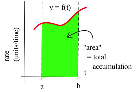
In our distance/velocity examples, the function represented a rate of travel (miles per hour), and the area represented the total distance traveled. This principle works more generally:
For functions representing other rates such as the production of a factory (bicycles per day), or the flow of water in a river (gallons per minute) or traffic over a bridge (cars per minute), or the spread of a disease (newly sick people per week), the area will still represent the total amount of something.
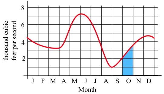
The graph below shows the flow rate (cubic feet per second) of water in the Skykomish river at the town of Goldbar in Washington state.
Solution
The area of the shaded region represents the total volume (cubic feet or \( \text{ft}^3 \)) of water flowing past the town during the month of October. We can approximate this area to approximate the total water by thinking of the shaded region as a rectangle with a triangle on top.
\[ \begin{align*} \text{Total water } & = \text{ total area}\\ & \approx \text{ area of rectangle }+\text{ area of the "triangle"} \\ & \approx \left(2000 \frac{\text{ft}^3}{\text{s}}\right)\left(30 \text{ days}\right)+\frac{1}{2}\left(1500\frac{\text{ft}^3}{\text{s}}\right)\left(30\text{ days}\right) \\ & = \left(2570\frac{\text{ft}^3}{\text{s}}\right)\left(30\text{ days}\right) \end{align*} \nonumber \]
Note that we need to convert the units to make sense of our result: \[ \begin{align*} \text{Total water } & \approx \left(2570\frac{\text{ft}^3}{\text{s}}\right)\left(30\text{ days}\right) \\ & = \left(2570\frac{\text{ft}^3}{\text{s}}\right)\left(2,\!592,\!000\text{ sec}\right) \\ & \approx 7.128\cdot 10^9\text{ ft}^3 \end{align*} \nonumber \]
About 7 billion cubic feet of water flowed past Goldbar in October.
Approximating with Rectangles
How do we approximate the area if the rate curve is, well, curvy
? We could use rectangles and triangles, like we did in the last example. But it turns out to be more useful (and easier) to simply use rectangles. The more rectangles we use, the better our approximation is.
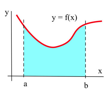
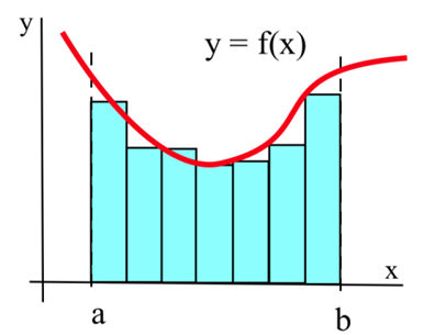
Suppose we want to calculate the area between the graph of a positive function \(f\) and the \(x\)-axis on the interval \([a, b]\) (graphed above). The Riemann Sum method is to build several rectangles with bases on the interval \([a, b]\) and sides that reach up to the graph of \(f\) (see below). Then the areas of the rectangles can be calculated and added together to get a number called a Riemann Sum of \(f\) on \([a, b]\). The area of the region formed by the rectangles is an approximation of the area we want.
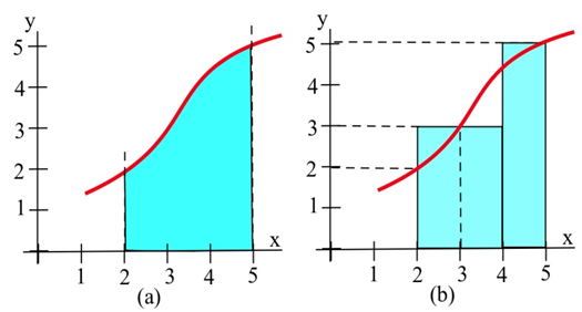
Approximate the area in the graph on the left between the graph of \(f\) and the \(x\)-axis on the interval [2, 5] by summing the areas of the rectangles in the graph on the right.
Solution
The total area of rectangles is \[(2)(3) + (1)(5) = 11\text{ units}^2.\nonumber \]
Let \(A\) be the region bounded by the graph of \(f(x) = \frac{1}{x}\), the \(x\)-axis, and vertical lines at \(x = 1\) and \(x = 5\). We can’t find the area exactly (with what we know now), but we can approximate it using rectangles.
When we make our rectangles, we have a lot of choices. We could pick any (non-overlapping) rectangles whose bottoms lie within the interval on the x-axis, and whose tops intersect with the curve somewhere. But it is easiest to choose rectangles that (a) have all the same width and (b) take their heights from the function at one edge. Below are graphs showing two ways to use four rectangles to approximate this area. In the first graph, we used left-endpoints; the height of each rectangle comes from the function value at its left edge. In the second graph on the next page, we used right-hand endpoints.
Left-hand endpoints: The area is approximately the sum of the areas of the rectangles. Each rectangle gets its height from the function \( f(x)=\frac{1}{x} \) and each rectangle has a width of 1.
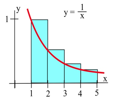
You can find the area of each rectangle using area = height\( \cdot \)width. So the total area of the rectangles, the left-hand estimate of the area under the curve, is \[f(1)\cdot 1+f(2)\cdot 1+f(3)\cdot 1+f(4)\cdot 1=1+\frac{1}{2}+\frac{1}{3}+\frac{1}{4}=\frac{25}{12}\approx 2.08.\nonumber \]
Notice that because this function is decreasing, all the left endpoint rectangles stick out above the region we want – using left-hand endpoints will overestimate the area.
Right-hand endpoints: The right-hand estimate of the area is \[f(2)\cdot 1+f(3)\cdot 1+f(4)\cdot 1+f(5)\cdot 1=\frac{1}{2}+\frac{1}{3}+\frac{1}{4}+\frac{1}{5}=\frac{77}{60}\approx 1.28.\nonumber \]

All the right-hand rectangles lie completely under the curve, so this estimate will be an underestimate.
We can see that the true area is actually in between these two estimates. So we could take their average: \[\text{Average}=\frac{\frac{25}{12}+\frac{77}{60}}{2}=\frac{101}{60}\approx 1.68\nonumber \]
In general, the average of the left-hand and right-hand estimates will be closer to the real area than either individual estimate.
Our estimate of the area under the curve is about 1.68. (The actual area is about 1.61.)
This applet will allow you to see how the approximation changes if you use more rectangles; change the position
slider to switch between using the left endpoints, right endpoints, and midpoints:
If we wanted a better answer, we could use even more and even narrower rectangles. But there is a limit to how much work we want to do by hand. In practice, choose a manageable number of rectangles. We will have better methods to get more accurate answers before long.
These sums of areas of rectangles are called Riemann sums. You may see a shorthand notation used when people talk about sums. We won't use it much in this book, but you should know what it means.
Riemann Sum
A Riemann sum for a function \(f(x)\) over an interval \([a, b]\) is a sum of areas of rectangles that approximates the area under the curve. Start by dividing the interval \([a, b]\) into \(n\) subintervals; each subinterval will be the base of one rectangle. We usually make all the rectangles the same width \( \Delta x \). The height of each rectangle comes from the function evaluated at some point in its sub interval. Then the Riemann sum is \[f(x_1)\Delta x+f(x_2)\Delta x+f(x_3)\Delta x+\dots +f(x_n)\Delta x\nonumber \] or, factoring out the \( \Delta x \), \[\Delta x\left(f(x_1)+f(x_2)+f(x_3)+\dots +f(x_n)\right).\nonumber \]
Sigma Notation
The upper-case Greek letter Sigma \( \sum \) is used to stand for sum
. Sigma notation is a way to compactly represent a sum of many similar terms, such as a Riemann sum.
Using the Sigma notation, the Riemann sum can be written \[\sum\limits_{i=1}^n f\left(x_i\right)\Delta x.\nonumber \]
This is read aloud as the sum as \(i\) goes from 1 to \(n\) of \(f\) of \(x\) sub \(i\) times Delta \(x\).
The \(i\)
is a counter or index, like you might have seen in a programming class.
Definition of the Definite Integral
Because the area under the curve is so important, it has a special vocabulary and notation.
The definite integral of a positive function \(f(x)\) over an interval \([a, b]\) is the area between \(f\), the \(x\)-axis, \(x = a\) and \(x = b\).
The definite integral of a positive function \(f(x)\) from \(a\) to \(b\) is the area under the curve between \(a\) and \(b\).
If \(f(t)\) represents a positive rate (in \(y\)-units per \(t\)-units), then the definite integral of \(f(t)\) from \(a\) to \(b\) is the total \(y\)-units that accumulate between \(t = a\) and \(t = b\).
Notation for the Definite Integral
The definite integral of \(f(x)\) from \(a\) to \(b\) is written \[\int_a^b f(x)\, dx.\nonumber \]
The \( \int \) symbol is called the integral sign; it is an elongated letter S, standing for sum
. (The \( \int \) corresponds to the \( \sum \) from the Riemann sum)
The \(dx\) on the end must be included! The \(dx\) tells what the variable is – in this example, the variable is \(x\). (The \(dx\) corresponds to the \( \Delta x \) from the Riemann sum)
The function \(f\) is called the integrand.
The \(a\) and \(b\) are called the limits of integration.
Verb forms
We integrate, or find the definite integral of a function. This process is called integration.
Formal Algebraic Definition
\[\int_a^b f(x)\, dx =\lim\limits_{n\to\infty}\sum\limits_{i=1}^n f(x_i)\Delta x.\nonumber \]
Practical Definition
The definite integral can be approximated with a Riemann sum (dividing the area into rectangles where the height of each rectangle comes from the function, computing the area of each rectangle, and adding them up). The more rectangles we use, the narrower the rectangles are, the better our approximation will be.
Looking Ahead
We will have methods for computing exact values of some definite integrals from formulas soon. In many cases, including when the function is given to you as a table or graph, you will still need to approximate the definite integral with rectangles.
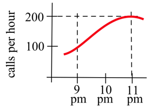
The graph below shows \(y = r(t)\), the number of telephone calls made per hours on a Tuesday. Approximately how many calls were made between 9 pm and 11 pm? Express this as a definite integral and approximate with a Riemann sum.
Solution
We know that the accumulated calls will be the area under this rate graph over that two-hour period, the definite integral of this rate from \(t = 9\) to \(t = 11\).
The total number of calls will be \( \int\limits_9^{11} r(t)\,dt \).
The top here is a curve, so we can’t get an exact answer. But we can approximate the area using rectangles. Let's choose to use four rectangles and left-endpoints:
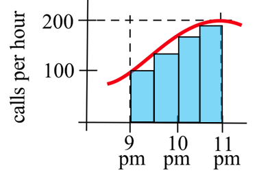
\[\int\limits_9^{11} r(t)\,dt \approx 0.5(100+150+180+195)=312.5\nonumber \]
The units are calls per hour\( \cdot \)hours = calls. Our estimate is that about 312 calls were made between 9 pm and 11 pm. Is this an under-estimate or an over-estimate?
Describe the area between the graph of \(f(x) = \frac{1}{x}\), the \(x\)-axis, and the vertical lines at \(x = 1\) and \(x = 5\) as a definite integral.
Solution
This is the same area we estimated to be about 1.68 before. Now we can use the notation of the definite integral to describe it. Our estimate of \( \int\limits_1^5 \frac{1}{x}\, dx \) was 1.68. The true value of \( \int\limits_1^5 \frac{1}{x}\, dx \) is about 1.61.
Using the idea of area, determine the value of \( \int\limits_1^3 1+x \,dx \).
Solution
\( \int\limits_1^3 1+x \,dx \) represents the area between the graph of \(f(x) = 1+x\), the \(x\)-axis, and the vertical lines at 1 and 3.
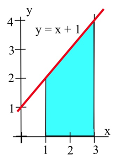
Since this area can be broken into a rectangle and a triangle, we can find the area exactly. The area equals \[ 4 + \frac{1}{2}(2)(2) = 6 \text{ units}^2.\nonumber \]
The table shows rates of population growth for Berrytown for several years. Use this table to estimate the total population growth from 1970 to 2000:
| Year, \( t \) | 1970 | 1980 | 1990 | 2000 |
| Rate of population growth \( R(t) \) in thousands of people per year | 1.5 | 1.9 | 2.2 | 2.4 |
Solution
The definite integral of this rate will give the total change in population over the thirty-year period. We only have a few pieces of information, so we can only estimate. Even though we haven't made a graph, we're still approximating the area under the rate curve, using rectangles. How wide are the rectangles? We have information every 10 years, so the rectangles have a width of 10 years. How many rectangles? Be careful here – this is a thirty-year span, so there are three rectangles.
- Using left-hand endpoints: (1.5)(10) + (1.9)(10) + (2.2)(10) = 56
- Using right-hand endpoints: (1.9)(10) + (2.2)(10) + (2.4)(10) = 65
Taking the average of these two: \[\frac{56+65}{2}=60.5\nonumber \]
Our best estimate of the total population growth from 1970 to 2000 is 60.5 thousand people.
Signed Area
You may have noticed that until this point, we've insisted that the integrand (the function we're integrating) be positive. That’s because we've been talking about area, which is always positive.
If the height
(from the function) is a negative number, then multiplying it by the width doesn't give us actual area, it gives us the area with a negative sign.
But it turns out to be useful to think about the possibility of negative area. We’ll expand our idea of a definite integral now to include integrands that might not always be positive. The heights
of the rectangles, the values from the function, now might not always be positive.
The definite integral of a function \(f(x)\) over an interval \([a, b]\) is the signed area between \(f\), the \(x\)-axis, \(x = a\) and \(x = b\).
The definite integral of a function \(f(x)\) from \(a\) to \(b\) is the signed area under the curve between \(a\) and \(b\).
If the function is positive, the signed area is positive, as before (and we can call it area.)
If the function dips below the \(x\)-axis, the areas of the regions below the \(x\)-axis come in with a negative sign. In this case, we cannot call it simply area.
These negative areas take away from the definite integral.
\( \int\limits_a^b f(x) \,dx = \) (Area above \( x \)-axis) \( - \) (Area below \( x \)-axis)
If \(f(t)\) represents a positive rate (in \(y\)-units per \(t\)-units), then the definite integral of \(f\) from \(a\) to \(b\) is the total \(y\)-units that accumulate between \(t = a\) and \(t = b\).
If \(f(t)\) represents any rate (in \(y\)-units per \(t\)-units), then the definite integral of \(f\) from \(a\) to \(b\) is the net \(y\)-units that accumulate between \(t = a\) and \(t = b\).
Find the definite integral of \(f(x) = –2\) on the interval [1,4].
Solution
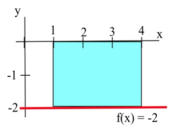
\(\int\limits_1^4 -2\,dx\) is the signed area of the region shown to the right. The region lies below the \( x \)-axis, so the area, 6, comes in with a negative sign. So the definite integral is \(\int\limits_1^4 -2\,dx =-6\).
Negative rates indicate that the amount is decreasing. For example, if \(f(t)\) is the velocity of a car in the positive direction along a straight line at time \(t\) (miles/hour), then negative values of \(f\) indicate that the car is traveling in the negative direction, backwards. The definite integral of \(f\) is the change in position of the car during the time interval. If the velocity is positive, positive distance accumulates. If the velocity is negative, distance in the negative direction accumulates.
This is true of any rate. For example, if \(f(t)\) is the rate of population change (people/year) for a town, then negative values of \(f\) would indicate that the population of the town was getting smaller, and the definite integral (now a negative number) would be the change in the population, a decrease, during the time interval.
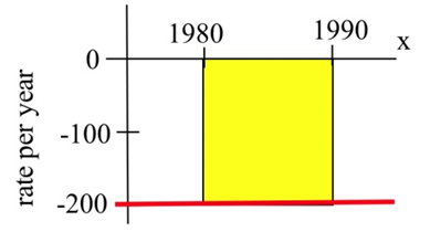
In 1980 there were 12,000 ducks nesting around a lake, and the rate of population change (in ducks per year) is shown in the figure below. Write a definite integral to represent the total change in the duck population from 1980 to 1990, and estimate the population in 1990.
Solution
The change in population is: \[ \begin{align*} \int\limits_{1980}^{1990} f(t) \,dt & = -(\text{area between \( f \) and axis}) \\ & \approx -(200\text{ ducks/year})\cdot (10\text{ years}) \\ & = -2000\text{ ducks} \end{align*} \nonumber \]
Then (1990 duck population) = (1980 population) + (change from 1980 to 1990) = (12,000) + ( -2000) = 10,000 ducks.
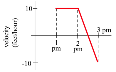
A bug starts at the location \(x = 12\) on the \(x\)-axis at 1 pm walks along the axis with the velocity \(v(x)\) shown in the graph. How far does the bug travel between 1 pm and 3 pm, and where is the bug at 3 pm?
Solution
Note that the velocity is positive from 1 until 2:30, then becomes negative. So the bug moves in the positive direction from 1 until 2:30, then turns around and moves back toward where it started. The area under the velocity curve from 1 to 2:30 shows the total distance traveled by the bug in the positive direction; the bug moved 12.5 feet in the positive direction. The area between the velocity curve and the x-axis, between 2:30 and 3, shows the total distance traveled by the bug in the negative direction, back toward home; the bug traveled 2.5 feet in the negative direction. The definite integral of the velocity curve, \(\int\limits_1^3 v(t) \,dt\), shows the net change in distance: \[\int\limits_1^3 v(t) \,dt = 12.5-2.5=10.\nonumber \]
The bug ended up 10 feet farther in the positive direction than he started. At 3 pm, the bug is at \(x = 22\).
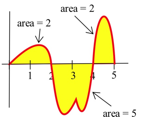
Use the graph below to calculate \( \int\limits_0^2 f(x) \,dx \), \( \int\limits_2^4 f(x) \,dx \), \( \int\limits_4^5 f(x) \,dx \), and \( \int\limits_0^5 f(x) \,dx \).
Solution
Using the given areas, \( \int\limits_0^2 f(x) \,dx = 2 \), \( \int\limits_2^4 f(x) \,dx = -5 \), \( \int\limits_4^5 f(x) \,dx = 2 \), and \( \int\limits_0^5 f(x) \,dx = \)(area above)\( - \)(area below)\( = (2+2) - (5) = -1\).
Approximating with Technology
If your function is given as a graph or table, you will still have to approximate definite integrals using areas, usually of rectangles. But if your function is given as a formula, you can turn to technology to get a better approximate answer. For example, most graphing calculators have some kind of numerical integration tool built in. You can also find many online tools that can do this; type numerical integration into any search engine to see a selection of these.
Most numerical integration tools use rectangles to estimate the signed area, just as you would do by hand. But they use many more rectangles than you would have the patience for, so they get a better answer. Some of them use computer algebra systems to find exact answers; we will learn how to do this ourselves later in this chapter.
When you turn to technology to find the value of a definite integral, be careful. Not every tool will be able to give you a correct answer for every integral. You should make an estimate of the answer yourself first so you can judge whether the answer you get makes sense.
Use technology to approximate the definite integral \( \int\limits_1^5 \frac{1}{x} \,dx \). (This is the same definite integral we approximated with rectangles before.)
Solution
We could use the following command in GeoGebra to approximate this integral:
Integral[1 / x, 1, 5]
Or click this link to see how to evaluate this integral using Wolfram|Alpha.
Use technology to approximate the definite integral \( \int\limits_1^2 e^{x^2+x} \,dx \).
Solution
The function here is positive, so there must be some area under the curve here. There isn’t an algebraic way to find the exact answer, so some programs may just return the original integral rather than try to approximate it.
We could use the following command in GeoGebra to approximate this integral:
Integral[e^(x^2 + x), 1, 2]
Or click this link to see how to approximate this integral using Wolfram|Alpha. Although it looks like Wolfram|Alpha can evaluate the integral, the Erfi
function that it shows in its answer is actually defined in terms of another integral, so it still hasn't found an algebraic answer.
Accumulation in Real Life
We have already seen that the area
under a graph can represent quantities whose units are not the usual geometric units of square meters or square feet. For example, if \(t\) is a measure of time in seconds and \(f(t)\) is a velocity with units feet/second, then the definite integral has units (feet/second)\( \cdot \)(seconds) = feet.
In general, the units for the definite integral \( \int\limits_a^b f(x)\,dx \) are (\(y\)-units )\( \cdot \)(\(x\)-units). A quick check of the units can help avoid errors in setting up an applied problem.
In previous examples, we looked at a function that represented a rate of travel (miles per hour); in that case, the area represented the total distance traveled. For functions representing other rates such as the production of a factory (bicycles per day), or the flow of water in a river (gallons per minute) or traffic over a bridge (cars per minute), or the spread of a disease (newly sick people per week), the area will still represent the total amount of something.
Suppose \(MR(q)\) is the marginal revenue in dollars/item for selling \(q\) items. What does \( \int\limits_0^{150} MR(q) \,dq \) represent?
Solution
\( \int\limits_0^{150} MR(q) \,dq \) has units (dollars/item)\( \cdot \)(items) = dollars, and represents the accumulated dollars for selling from 0 to 150 items. That is, \( \int\limits_0^{150} MR(q) \,dq = TR(150) \), the total revenue from selling 150 items.
Suppose \(r(t)\), in centimeters per year, represents how the diameter of a tree changes with time. What does \( \int\limits_{T_1}^{T_2} r(t) \,dt \) represent?
Solution
\( \int\limits_{T_1}^{T_2} r(t) \,dt \) has units of (centimeters per year)\( \cdot \)(years) = centimeters, and represents the accumulated growth of the tree’s diameter from \(T_1\) to \(T_2\). That is, \( \int\limits_{T_1}^{T_2} r(t) \,dt \) is the change in the diameter of the tree over this period of time.