
11.4: Unit Tangent and Normal Vectors


- Last updated
- Dec 29, 2020
- Save as PDF

( \newcommand{\kernel}{\mathrm{null}\,}\)
Unit Tangent Vector
Given a smooth vector-valued function ⇀r(t), we defined in Definition 71 that any vector parallel to ⇀r′(t0) is tangent to the graph of ⇀r(t) at t=t0. It is often useful to consider just the direction of ⇀r′(t) and not its magnitude. Therefore we are interested in the unit vector in the direction of ⇀r′(t). This leads to a definition.
Definition 11.4.1: Unit Tangent Vector
Let ⇀r(t) be a smooth function on an open interval I. The unit tangent vector ⇀T(t) is
⇀T(t)=1‖⇀r′(t)‖⇀r′(t).
Example 11.4.1: Computing the unit tangent vector
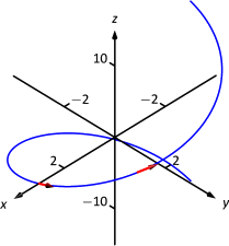
Let ⇀r(t)=⟨3cost,3sint,4t⟩. Find ⇀T(t) and compute ⇀T(0) and ⇀T(1).
Solution
We apply Definition 11.4.1 to find ⇀T(t).
⇀T(t)=1‖⇀r′(t)‖⇀r′(t)=1√(−3sint)2+(3cost)2+42⟨−3sint,3cost,4⟩=⟨−35sint,35cost,45⟩.
We can now easily compute ⇀T(0) and ⇀T(1):
⇀T(0)=⟨0,35,45⟩⇀T(1)=⟨−35sin1,35cos1,45⟩≈⟨−0.505,0.324,0.8⟩.
These are plotted in Figure 11.4.1 with their initial points at ⇀r(0) and ⇀r(1), respectively. (They look rather "short'' since they are only length 1.)
The unit tangent vector ⇀T(t) always has a magnitude of 1, though it is sometimes easy to doubt that is true. We can help solidify this thought in our minds by computing ‖⇀T(1)‖:
‖⇀T(1)‖≈√(−0.505)2+0.3242+0.82=1.000001.
We have rounded in our computation of ⇀T(1), so we don't get 1 exactly. We leave it to the reader to use the exact representation of ⇀T(1) to verify it has length 1.
In many ways, the previous example was "too nice.'' It turned out that ⇀r′(t) was always of length 5. In the next example the length of ⇀r′(t) is variable, leaving us with a formula that is not as clean.
Example 11.4.2: Computing the unit tangent vector
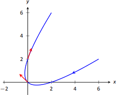
Let ⇀r(t)=⟨t2−t,t2+t⟩. Find ⇀T(t) and compute ⇀T(0) and ⇀T(1).
Solution
We find ⇀r′(t)=⟨2t−1,2t+1⟩, and
‖⇀r′(t)‖=√(2t−1)2+(2t+1)2=√8t2+2.
Therefore
⇀T(t)=1√8t2+2⟨2t−1,2t+1⟩=⟨2t−1√8t2+2,2t+1√8t2+2⟩.
When t=0, we have ⇀T(0)=⟨−1/√2,1/√2⟩; when t=1, we have ⇀T(1)=⟨1/√10,3/√10⟩. We leave it to the reader to verify each of these is a unit vector. They are plotted in Figure 11.4.2.
Unit Normal Vector
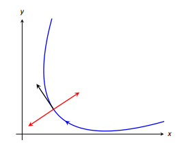
Just as knowing the direction tangent to a path is important, knowing a direction orthogonal to a path is important. When dealing with real-valued functions, we defined the normal line at a point to the be the line through the point that was perpendicular to the tangent line at that point. We can do a similar thing with vector-valued functions. Given ⇀r(t) in R2, we have 2 directions perpendicular to the tangent vector, as shown in Figure 11.4.3. It is good to wonder "Is one of these two directions preferable over the other?''
Given ⇀r(t) in R3, there are infinite vectors orthogonal to the tangent vector at a given point. Again, we might wonder "Is one of these infinite choices preferable over the others? Is one of these the "right' choice?''
The answer in both R2 and R3 is "Yes, there is one vector that is not only preferable, it is the "right' one to choose.'' Recall Theorem 93, which states that if ⇀r(t) has constant length, then ⇀r(t) is orthogonal to ⇀r′(t) for all t. We know ⇀T(t), the unit tangent vector, has constant length. Therefore ⇀T(t) is orthogonal to ⇀T′(t).
We'll see that ⇀T′(t) is more than just a convenient choice of vector that is orthogonal to ⇀r′(t); rather, it is the "right'' choice. Since all we care about is the direction, we define this newly found vector to be a unit vector.
Note: ⇀T(t) is a unit vector, by definition. This does not imply that ⇀T′(t) is also a unit vector.
Definition 11.4.2: Unit Normal Vector
Let ⇀r(t) be a vector-valued function where the unit tangent vector, ⇀T(t), is smooth on an open interval I. The unit normal vector ⇀N(t) is
⇀N(t)=1‖⇀T′(t)‖⇀T′(t).
Example 11.4.3: Computing the unit normal vector
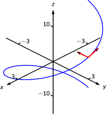
Let ⇀r(t)=⟨3cost,3sint,4t⟩ as in Example 11.4.1. Sketch both ⇀T(π/2) and ⇀N(π/2) with initial points at ⇀r(π/2).
Solution
In Example 11.4.1, we found ⇀T(t)=⟨(−3/5)sint,(3/5)cost,4/5⟩. Therefore
⇀T′(t)=⟨−35cost,−35sint,0⟩and‖⇀T′(t)‖=35.
Thus
⇀N(t)=⇀T′(t)3/5=⟨−cost,−sint,0⟩.
We compute ⇀T(π/2)=⟨−3/5,0,4/5⟩ and ⇀N(π/2)=⟨0,−1,0⟩. These are sketched in Figure 11.4.4.
The previous example was once again "too nice.'' In general, the expression for ⇀T(t) contains fractions of square-roots, hence the expression of ⇀T′(t) is very messy. We demonstrate this in the next example.
Example 11.4.4: Computing the unit normal vector
Let ⇀r(t)=⟨t2−t,t2+t⟩ as in Example 11.4.2. Find ⇀N(t) and sketch ⇀r(t) with the unit tangent and normal vectors at t=−1,0 and 1.
Solution
In Example 11.4.2, we found
⇀T(t)=⟨2t−1√8t2+2,2t+1√8t2+2⟩.
Finding ⇀T′(t) requires two applications of the Quotient Rule:
T′(t)=⟨√8t2+2(2)−(2t−1)(12(8t2+2)−1/2(16t))8t2+2,√8t2+2(2)−(2t+1)(12(8t2+2)−1/2(16t))8t2+2⟩=⟨4(2t+1)(8t2+2)3/2,4(1−2t)(8t2+2)3/2⟩
This is not a unit vector; to find ⇀N(t), we need to divide ⇀T′(t) by it's magnitude.
‖⇀T′(t)‖=√16(2t+1)2(8t2+2)3+16(1−2t)2(8t2+2)3=√16(8t2+2)(8t2+2)3=48t2+2.
Finally,
⇀N(t)=14/(8t2+2)⟨4(2t+1)(8t2+2)3/2,4(1−2t)(8t2+2)3/2⟩=⟨2t+1√8t2+2,−2t−1√8t2+2⟩.
Using this formula for ⇀N(t), we compute the unit tangent and normal vectors for t=−1,0 and 1 and sketch them in Figure 11.4.5.
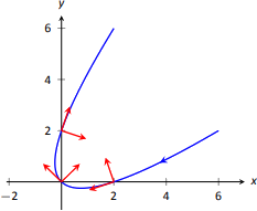
The final result for ⇀N(t) in Example 11.4.4 is suspiciously similar to ⇀T(t). There is a clear reason for this. If ⇀u=⟨u1,u2⟩ is a unit vector in R2, then the only unit vectors orthogonal to ⇀u are ⟨−u2,u1⟩ and ⟨u2,−u1⟩. Given ⇀T(t), we can quickly determine ⇀N(t) if we know which term to multiply by (−1).
Consider again Figure 11.24, where we have plotted some unit tangent and normal vectors. Note how ⇀N(t) always points "inside'' the curve, or to the concave side of the curve. This is not a coincidence; this is true in general. Knowing the direction that ⇀r(t) "turns'' allows us to quickly find ⇀N(t).
THEOREM 11.4.1: Unit Normal Vectors in R2
Let ⇀r(t) be a vector-valued function in R2 where ⇀T′(t) is smooth on an open interval I. Let t0 be in I and ⇀T(t0)=⟨t1,t2⟩ Then ⇀N(t0) is either
⇀N(t0)=⟨−t2,t1⟩or⇀N(t0)=⟨t2,−t1⟩,
whichever is the vector that points to the concave side of the graph of \vecs r.
Application to Acceleration
Let \vecs r (t) be a position function. It is a fact (stated later in Theorem \PageIndex{2}) that acceleration, \vecs a (t), lies in the plane defined by \vecs T and \vecs N. That is, there are scalars a_{\text{T}} and a_{\text{N}} such that
\vecs a (t) = a_{\text{T}}\vecs T(t) + a_{\text{N}}\vecs N(t).
The scalar a_{\text{T}} measures "how much'' acceleration is in the direction of travel, that is, it measures the component of acceleration that affects the speed. The scalar a_{\text{N}} measures "how much'' acceleration is perpendicular to the direction of travel, that is, it measures the component of acceleration that affects the direction of travel.
We can find a_{\text{T}} using the orthogonal projection of \vecs a(t) onto \vecs T(t) (review Definition 59 in Section 10.3 if needed).
Recalling that since \vecs T(t) is a unit vector, \vecs T(t)\cdot\vecs T(t)=1, so we have
\text{proj}_{T(t)}\vecs a(t) = \dfrac{\vecs a(t)\cdot\vecs T(t)}{\vecs T(t)\cdot\vecs T(t)}\vecs T(t) = \underbrace{\left(\vecs a(t)\cdot\vecs T(t)\right) }_{a_{\text{T}}}\vecs T(t).
Thus the amount of \vecs a (t) in the direction of \vecs T(t) is a_{\text{T}}=\vecs a (t)\cdot\vecs T(t). The same logic gives a_{\text{N}} = \vecs a (t)\cdot\vecs N(t).
While this is a fine way of computing a_{\text{T}}, there are simpler ways of finding a_{\text{N}} (as finding \vecs N itself can be complicated). The following theorem gives alternate formulas for a_{\text{T}} and a_{\text{N}}.
Note: Keep in mind that both a_\text{T} and a_\text{N} are functions of t; that is, the scalar changes depending on t. It is convention to drop the "(t)'' notation from a_\text{T}(t) and simply write a_\text{T}.
THEOREM \PageIndex{2}: Acceleration in the Plane Defined by \vecs T and \vecs N
Let \vecs r (t) be a position function with acceleration \vecs a (t) and unit tangent and normal vectors \vecs T(t) and \vecs N(t). Then \vecs a (t) lies in the plane defined by \vecs T(t) and \vecs N(t); that is, there exists scalars a_\text{T} and a_\text{N} such that
\vecs a (t) = a_\text{T}\vecs T(t) + a_\text{N}\vecs N(t).
Moreover,
\begin{align*} a_\text{T} &= \vecs a (t)\cdot\vecs T(t) = \dfrac{d}{dt}\left(\norm{\vecs v(t)}\right) \\[4pt] a_\text{N} &= \vecs a (t)\cdot \vecs N(t) = \sqrt{\norm{\vecs a(t)}^2-a_\text{T}^2} = \dfrac{\norm{\vecs a (t)\times\vecs v (t)}}{\norm{\vecs v (t)}} = \norm{\vecs v (t)}\,\norm{\vecs T\,'(t)} \end{align*}
Note the second formula for a_\text{T}: \dfrac{d}{dt}\left(\norm{\vecs v (t)}\right) . This measures the rate of change of speed, which again is the amount of acceleration in the direction of travel.
Example \PageIndex{5}: Computing a_\text{T} and a_\text{N}
Let \vecs r (t) = \langle 3\cos t, 3\sin t, 4t\rangle as in Examples 11.4.1 and 11.4.3. Find a_\text{T} and a_\text{N}.
Solution
The previous examples give \vecs a (t) = \langle -3\cos t,-3\sin t,0\rangle and
\vecs T(t) = \langle -\dfrac35\sin t,\dfrac35\cos t,\dfrac45\rangle \quad \text{and}\quad \vecs N(t) = \langle -\cos t,-\sin t,0\rangle.
We can find a_\text{T} and a_\text{N} directly with dot products:
\begin{align*} a_\text{T} &= \vecs a (t)\cdot \vecs T(t) = \dfrac95\cos t\sin t-\dfrac95\cos t\sin t+0 = 0.\\[4pt] a_\text{N} &= \vecs a (t)\cdot \vecs N(t) = 3\cos^2t+3\sin^2t + 0 = 3. \end{align*}
Thus \vecs a (t) = 0\vecs T(t) + 3\vecs N(t) = 3\vecs N(t), which is clearly the case.
What is the practical interpretation of these numbers? a_\text{T}=0 means the object is moving at a constant speed, and hence all acceleration comes in the form of direction change.
Example \PageIndex{6}: Computing a_\text{T} and a_\text{N}
Let \vecs r (t)=\langle t^2-t,t^2+t\rangle as in Examples \PageIndex{2} and \PageIndex{4}. Find a_\text{T} and a_\text{N}.
Solution
The previous examples give \vecs a(t) = \langle 2,2\rangle and
\vecs T(t) = \langle \dfrac{2t-1}{\sqrt{8t^2+2}},\dfrac{2t+1}{\sqrt{8t^2+2}}\rangle \nonumber
and
\vecs N(t) = \langle \dfrac{2t+1}{\sqrt{8t^2+2}},-\dfrac{2t-1}{\sqrt{8t^2+2}}\rangle. \nonumber
While we can compute a_\text{N} using \vecs N(t), we instead demonstrate using another formula from Theorem \PageIndex{2}.
\begin{align*} a_\text{T} &= \vecs a (t)\cdot\vecs T(t) = \dfrac{4t-2}{\sqrt{8t^2+2}}+\dfrac{4t+2}{\sqrt{8t^2+2}} = \dfrac{8t}{\sqrt{8t^2+2}}.\\[4pt] a_\text{N} &= \sqrt{\norm{\vecs a (t)}^2-a_\text{T}^2} = \sqrt{8-\left(\dfrac{8t}{\sqrt{8t^2+2}}\right)^2}=\dfrac{4}{\sqrt{8t^2+2}} \end{align*}
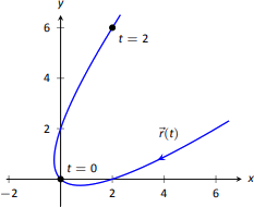
When t=2, a_\text{T} = \dfrac{16}{\sqrt{34}}\approx 2.74 and a_\text{N} = \dfrac{4}{\sqrt{34}} \approx 0.69. We interpret this to mean that at t=2, the particle is accelerating mostly by increasing speed, not by changing direction. As the path near t=2 is relatively straight, this should make intuitive sense. Figure \PageIndex{6} gives a graph of the path for reference.
Contrast this with t=0, where a_\text{T} = 0 and a_\text{N} = 4/\sqrt{2}\approx 2.82. Here the particle's speed is not changing and all acceleration is in the form of direction change.
Example \PageIndex{7}: Analyzing projectile motion
A ball is thrown from a height of 240ft with an initial speed of 64ft/s and an angle of elevation of 30^\circ. Find the position function \vecs r (t) of the ball and analyze a_\text{T} and a_\text{N}.
Solution
Using Key Idea 53 of Section 11.3 we form the position function of the ball:
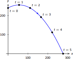
\vecs r (t) = \langle \left(64\cos 30^\circ\right) t, -16t^2+\left(64\sin 30^\circ\right) t+240\rangle,
which we plot in Figure \PageIndex{7}.
From this we find \vecs v (t) = \langle 64\cos 30^\circ, -32t+64\sin 30^\circ\rangle and \vecs a (t) = \langle 0,-32\rangle. Computing \vecs T(t) is not difficult, and with some simplification we find
\vecs T(t) = \langle \dfrac{\sqrt{3}}{\sqrt{t^2-2t+4}}, \dfrac{1-t}{\sqrt{t^2-2t+4}}\rangle.
With \vecs a (t) as simple as it is, finding a_\text{T} is also simple:
a_\text{T} = \vecs a (t)\cdot \vecs T(t) = \dfrac{32t-32}{\sqrt{t^2-2t+4}}.
We choose to not find \vecs N(t) and find a_\text{N} through the formula a_\text{N} = \sqrt{\norm{\vecs a (t)}^2-a_\text{T}^2\,}:
a_\text{N} = \sqrt{32^2-\left(\dfrac{32t-32}{\sqrt{t^2-2t+4}}\right)^2} = \dfrac{32\sqrt{3}}{\sqrt{t^2-2t+4}}.
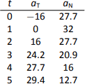
Figure \PageIndex{8} gives a table of values of a_\text{T} and a_\text{N}. When t=0, we see the ball's speed is decreasing; when t=1 the speed of the ball is unchanged. This corresponds to the fact that at t=1 the ball reaches its highest point.
After t=1 we see that a_\text{N} is decreasing in value. This is because as the ball falls, it's path becomes straighter and most of the acceleration is in the form of speeding up the ball, and not in changing its direction.
Our understanding of the unit tangent and normal vectors is aiding our understanding of motion. The work in Example \PageIndex{7} gave quantitative analysis of what we intuitively knew.
The next section provides two more important steps towards this analysis. We currently describe position only in terms of time. In everyday life, though, we often describe position in terms of distance ("The gas station is about 2 miles ahead, on the left.''). The arc length parameter allows us to reference position in terms of distance traveled.
We also intuitively know that some paths are straighter than others - and some are "curvier" than others, but we lack a measurement of "curviness.'' The arc length parameter provides a way for us to compute curvature, a quantitative measurement of how curvy a curve is.