3.E: Multiple Integrals (Exercises)

3.1: Double Integrals

A

For Exercises 1-4, find the volume under the surface \(z = f (x, y)\) over the rectangle \(R\).

3.1.1. \(f (x, y) = 4x y,\, R = [0,1]×[0,1] \)

3.1.2. \(f (x, y) = e^{ x+y} ,\, R = [0,1]×[−1,1] \)

3.1.3. \(f (x, y) = x^ 3 + y^ 2 ,\, R = [0,1]×[0,1] \)

3.1.4. \(f (x, y) = x^ 4 + x y+ y^ 3 ,\, R = [1,2]×[0,2]\)

For Exercises 5-12, evaluate the given double integral.

3.1.5. \(\int_0^1 \int_1^2 (1− y)x^ 2 \,dx \,d y\)

3.1.6. \(\int_0^1 \int_0^2 x(x+ y)\,dx \,d y\)

3.1.7. \(\int_0^2 \int_0^1 (x+2)\,dx \,d y\)

3.1.8. \(\int_{−1}^2 \int_{−1}^1 x(x y+\sin x)\,dx\, d y\)

3.1.9. \(\int_0^{\pi /2} \int_0^1 x y\cos (x^ 2 y)\,dx\, d y\)

3.1.10. \(\int_0^{\pi} \int_0^{π/2} \sin x \cos (y−π) \,dx\, d y\)

3.1.11. \(\int_0^2 \int_1^4 x y \,dx\, d y\)

3.1.12. \(\int_{-1}^1 \int_{-1}^2 1\,dx\, d y\)

3.1.13. Let \(M\) be a constant. Show that \(\int_c^d \int_a^b M\, dx \,d y = M(d − c)(b − a).\)

3.2: Double Integrals Over a General Region

A

For Exercises 1-6, evaluate the given double integral.

3.2.1. \(\int_0^1 \int_{\sqrt{ x}}^1 24x^ 2 y \,d y\, dx\)

3.2.2. \(\int_0^π \int_0^y \sin x \,dx\, d y\)

3.2.3. \(\int_1^2 \int_0^{\ln x} 4x \,d y\, dx\)

3.2.4. \(\int_0^2 \int_0^{2y} e^ {y^ 2} \,dx \,d y\)

3.2.5. \(\int_0^{π/2} \int_0^y \cos x \sin y \,dx \,d y\)

3.2.6. \(\int_0^{∞} \int_0^{∞} x ye^{−(x^ 2+y^ 2 )}\, dx \,d y\)

3.2.7. \(\int_0^2 \int_0^y 1\,dx \,d y\)

3.2.8. \(\int_0^1 \int_0^{x^ 2} 2\,d y\, dx\)

3.2.9. Find the volume \(V\) of the solid bounded by the three coordinate planes and the plane \(x+ y+ z = 1\).

3.2.10. Find the volume \(V\) of the solid bounded by the three coordinate planes and the plane \(3x+2y+5z = 6\).

B

3.2.11. Explain why the double integral \(\iint\limits_R 1\,d A\) gives the area of the region \(R\). For simplicity, you can assume that \(R\) is a region of the type shown in Figure 3.2.1(a).

C

3.2.12. Prove that the volume of a tetrahedron with mutually perpendicular adjacent sides of lengths \(a,\, b, \text{ and }c\), as in Figure 3.2.6, is \(\frac{abc}{ 6}\). (Hint: Mimic Example 3.5, and recall from Section 1.5 how three noncollinear points determine a plane.)

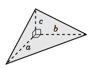
Figure 3.2.6

3.2.13. Show how Exercise 12 can be used to solve Exercise 10.

3.3: Triple Integrals

A

For Exercises 1-8, evaluate the given triple integral.

3.3.1. \(\int_0^3 \int_0^2 \int_0^1 x yz \,dx\, d y\, dz\)

3.3.2. \(\int_0^1 \int_0^x \int_0^y x yz \,dz\, d y\, dx\)

3.3.3. \(\int_0^π \int_0^x \int_0^{x y} x^ 2 \sin z \,dz\, d y\, dx\)

3.3.4. \(\int_0^1 \int_0^z \int_0^y ze^{ y^ 2} \,dx\, d y\, dz\)

3.3.5. \(\int_1^e \int_0^y \int_0^{1/y} x^ 2 z \,dx \,dz \,d y\)

3.3.6. \(\int_1^2 \int_0^{y^ 2} \int_0^{z^ 2} yz \,dx \,dz \,d y\)

3.3.7. \(\int_1^2 \int_2^4 \int_0^3 1\,dx \,d y\, dz\)

3.3.8. \(\int_0^1 \int_0^{1−x} \int_0^{1−x−y} 1\,dz\, d y\, dx\)

3.3.9. Let \(M\) be a constant. Show that \(\int_{z_1}^{z_2} \int_{y_1}^{y_2} \int_{x_1}^{x_2} M\, dx\, d y\, dz = M(z_2 − z_1)(y_2 − y_1)(x_2 − x_1)\).

B

3.3.10. Find the volume \(V\) of the solid \(S\) bounded by the three coordinate planes, bounded above by the plane \(x+ y+ z = 2\), and bounded below by the plane \(z = x+ y\).

C

3.3.11. Show that \(\int_a^b \int_a^z \int_a^y f (x)\,dx \,d y \,dz = \int_a^b \frac{(b−x)^ 2}{ 2} f (x)\,dx\). (Hint: Think of how changing the order of integration in the triple integral changes the limits of integration.)

3.4: Numerical Approximation of Multiple Integrals

C

3.4.1. Write a program that uses the Monte Carlo method to approximate the double integral \(\iint\limits_R e^{ x y}\, d A\), where \(R = [0,1]×[0,1]\). Show the program output for \(N = 10,\, 100,\, 1000,\, 10000,\, 100000 \text{ and }1000000\) random points.

3.4.2. Write a program that uses the Monte Carlo method to approximate the triple integral \iiint\limits_S e^{ x yz}\, dV\), where \(S = [0,1] × [0,1] × [0,1]\). Show the program output for \(N = 10,\, 100,\, 1000,\, 10000,\, 100000 \text{ and }1000000\) random points.

3.4.3. Repeat Exercise 1 with the region \(R = {(x, y) : −1 ≤ x ≤ 1,\, 0 ≤ y ≤ x^ 2 }\).

3.4.4. Repeat Exercise 2 with the solid \(S = {(x, y, z) : 0 ≤ x ≤ 1,\, 0 ≤ y ≤ 1, \,0 ≤ z ≤ 1− x− y}\).

3.4.5. Use the Monte Carlo method to approximate the volume of a sphere of radius 1.

3.4.6. Use the Monte Carlo method to approximate the volume of the ellipsoid \(\frac{x^ 2}{ 9} + \frac{y^ 2}{ 4} + \frac{z^ 2}{ 1} = 1\).

3.5: Change of Variables in Multiple Integrals

A

3.5.1. Find the volume \(V\) inside the paraboloid \(z = x^ 2 + y^ 2 \text{ for }0 ≤ z ≤ 4\).

3.5.2. Find the volume \(V\) inside the cone \(z = \sqrt{ x^ 2 + y^ 2}\) for \(0 ≤ z ≤ 3\).

B

3.5.3. Find the volume \(V\) of the solid inside both \(x^ 2 + y^ 2 + z^ 2 = 4\) and \(x^ 2 + y^ 2 = 1\).

3.5.4. Find the volume \(V\) inside both the sphere \(x^ 2 + y^ 2 + z^ 2 = 1\) and the cone \(z = \sqrt{ x^ 2 + y^ 2}\).

3.5.5. Prove Equation (3.25).

3.5.6. Prove Equation (3.26).

3.5.7. Evaluate \(\iiint\limits_R \sin \left ( \frac{x+y}{ 2} \right ) \cos \left ( \frac{x−y}{ 2} \right ) \,d A\), where \(R\) is the triangle with vertices \((0,0),\, (2,0) \text{ and }(1,1)\). (Hint: Use the change of variables \(u = (x+ y)/2,\, v = (x− y)/2.\))

3.5.8. Find the volume of the solid bounded by \(z = x^ 2 + y^ 2 \text{ and }z^ 2 = 4(x^ 2 + y^ 2 )\).

3.5.9. Find the volume inside the elliptic cylinder \(\frac{x^ 2}{ a^ 2} + \frac{y^ 2}{ b^ 2} = 1 \text{ for } 0 ≤ z ≤ 2\).

C

3.5.10. Show that the volume inside the ellipsoid \(\frac{x^ 2}{ a^ 2} + \frac{y^ 2}{ b^ 2} + \frac{z^ 2}{ c^ 2} = 1 \text{ is }\frac{4πabc}{ 3}\). (Hint: Use the change of variables \(x = au,\, y = bv,\, z = cw\), then consider Example 3.12.)

3.5.11. Show that the Beta function, defined by

\[B(x, y) = \int_0^1 t^{ x−1} (1− t)^{ y−1} dt ,\text{ for }x > 0,\, y > 0,\]

satisfies the relation \(B(y, x) = B(x, y) \text{ for }x > 0,\, y > 0.\)

3.5.12. Using the substitution \(t = u/(u +1)\), show that the Beta function can be written as

\[B(x, y) = \int_0^∞ \frac{u^{ x−1}}{ (u +1)^{x+y}}\, du ,\text{ for }x > 0,\, y > 0.\]

3.6: Application: Center of Mass

A

For Exercises 1-5, find the center of mass of the region \(R\) with the given density function \(δ(x, y)\).

3.6.1. \(R = {(x, y) : 0 ≤ x ≤ 2,\, 0 ≤ y ≤ 4 },\, δ(x, y) = 2y\)

3.6.2. \(R = {(x, y) : 0 ≤ x ≤ 1,\, 0 ≤ y ≤ x 2 },\, δ(x, y) = x+ y \)

3.6.3. \(R = {(x, y) : y ≥ 0,\, x^ 2 + y^ 2 ≤ a^ 2 },\, δ(x, y) = 1\)

3.6.4. \(R = {(x, y) : y ≥ 0,\, x ≥ 0,\, 1 ≤ x^ 2 + y^ 2 ≤ 4 },\, δ(x, y) = \sqrt{ x^ 2 + y^ 2}\)

3.6.5. \(R = {(x, y) : y ≥ 0,\, x^ 2 + y^ 2 ≤ 1 },\, δ(x, y) = y\)

B

For Exercises 6-10, find the center of mass of the solid \(S\) with the given density function \(δ(x, y, z)\).

3.6.6. \(S = {(x, y, z) : 0 ≤ x ≤ 1,\, 0 ≤ y ≤ 1,\, 0 ≤ z ≤ 1 },\, δ(x, y, z) = x yz\)

3.6.7. \(S = {(x, y, z) : z ≥ 0,\, x^ 2 + y^ 2 + z^ 2 ≤ a^ 2 },\, δ(x, y, z) = x^ 2 + y^ 2 + z^ 2\)

3.6.8. \(S = {(x, y, z) : x ≥ 0,\, y ≥ 0,\, z ≥ 0,\, x^ 2 + y^ 2 + z^ 2 ≤ a^ 2 },\, δ(x, y, z) = 1\)

3.6.9. \(S = {(x, y, z) : 0 ≤ x ≤ 1,\, 0 ≤ y ≤ 1,\, 0 ≤ z ≤ 1 },\, δ(x, y, z) = x^ 2 + y^ 2 + z^ 2\)

3.6.10. \(S = {(x, y, z) : 0 ≤ x ≤ 1,\, 0 ≤ y ≤ 1,\, 0 ≤ z ≤ 1− x− y},\, δ(x, y, z) = 1\)

3.7: Application: Probability and Expected Value

B

3.7.1. Evaluate the integral \(\int_{−\infty}^{\infty} e^{ −x^ 2}\, dx\) using anything you have learned so far.

3.7.2. For \(σ > 0 \text{ and }µ > 0\), evaluate \(\int_{\infty}^{−\infty} \frac{1}{ σ \sqrt{ 2π}} e^{ −(x−µ)^ 2 /2σ^ 2} dx\).

3.7.3. Show that \(EY = \frac{n}{ n+1}\) in Example 3.18

C

3.7.4. Write a computer program (in the language of your choice) that verifies the results in Example 3.18 for the case \(n = 3\) by taking large numbers of samples.

3.7.5. Repeat Exercise 4 for the case when \(n = 4\).

3.7.6. For continuous random variables \(X, Y \text{ with joint p.d.f. }f (x, y)\), define the second moments \(E(X^ 2 ) \text{ and }E(Y^ 2 )\) by

\[E(X^ 2 ) = \int_{-\infty}^{\infty} \int_{-\infty}^{\infty} x^ 2 f (x, y)\,dx\, d y \text{ and }E(Y^ 2 ) = \int_{-\infty}^{\infty} \int_{-\infty}^{\infty} y^ 2 f (x, y)\,dx \,d y ,\]

and the variances Var\((X)\) and Var\((Y)\) by

\[\text{Var}(X) = E(X^ 2 )−(EX)^ 2 \text{ and Var}(Y) = E(Y^ 2 )−(EY)^ 2 .\]

Find Var\((X)\) and Var\((Y)\) for \(X\) and \(Y\) as in Example 3.18.

3.7.7. Continuing Exercise 6, the correlation \(ρ \text{ between }X \text{ and }Y\) is defined as

\[ρ = \frac{E(XY)−(EX)(EY)}{ \sqrt{ \text{Var}(X)\text{Var}(Y)}} ,\]

where \(E(XY) = \int_{-\infty}^{\infty} \int_{-\infty}^{\infty} x y \,f (x, y)\,dx\, d y\). Find \(ρ\) for \(X \text{ and }Y\) as in Example 3.18.
(Note: The quantity \(E(XY)−(EX)(EY)\) is called the covariance of \(X\) and \(Y\).)

3.7.8. In Example 3.17 would the answer change if the interval \((0,100)\) is used instead of \((0,1)\)? Explain.

Contributors and Attributions

• Michael Corral (Schoolcraft College). The content of this page is distributed under the terms of the GNU Free Documentation License, Version 1.2.