1.12: Higher-Order Derivatives

Given two quantities, \(y\) and \(x,\) with \(y\) a function of \(x,\) we know that the derivative \(\frac{d y}{d x}\) is the rate of change of \(y\) with respect to \(x\). Since \(\frac{d y}{d x}\) is then itself a function of \(x,\) we may ask for its rate of change with respect to \(x,\) which we call the second-order derivative of \(y\) with respect to \(x\) and denote \(\frac{d^{2} y}{d x^{2}} .\)

Example \(\PageIndex{1}\)

If \(y=4 x^{5}-3 x^{2}+4,\) then

\[\frac{d y}{d x}=20 x^{4}-6 x ,\] and so \[\frac{d^{2} y}{d x^{2}}=80 x^{3}-6 .\] Of course, we could continue to differentiate: the third derivative of \(y\) with respect to \(x\) is \[\frac{d^{3} y}{d x^{3}}=240 x^{2} ,\] the fourth derivative of \(y\) with respect to \(x\) is \[\frac{d^{4} y}{d x^{4}}=480 x ,\] and so on.

If \(y\) is a function of \(x\) with \(y=f(x),\) then we may also denote the second derivative of \(y\) with respect to \(x\) by \(f^{\prime \prime}(x),\) the third derivative by \(f^{\prime \prime \prime}(x),\) and so on. The prime notation becomes cumbersome after awhile, and so we may replace the primes with the corresponding number in parentheses; that is, we may write, for example, \(f^{\prime \prime \prime \prime}(x)\) as \(f^{(4)}(x)\).

Example \(\PageIndex{2}\)

If

\[f(x)=\frac{1}{x} ,\] then \[\begin{aligned} f^{\prime}(x) &=-\frac{1}{x^{2}}, \\[12pt] f^{\prime \prime}(x) &=\frac{2}{x^{3}}, \\[12pt] f^{\prime \prime \prime}(x) &=-\frac{6}{x^{4}}, \end{aligned}\] and \[f^{(4)}(x)=\frac{24}{x^{5}} .\]

Exercise \(\PageIndex{1}\)

Find the first, second, and third-order derivatives of \(y=\sin (2 x)\).

Answer

\(\frac{d y}{d x}=2 \cos (2 x), \frac{d^{2} y}{d x^{2}}=-4 \sin (2 x), \frac{d^{3} y}{d x^{3}}=-8 \cos (2 x)\)

Exercise \(\PageIndex{2}\)

Find the first, second, and third-order derivatives of \(f(x)=\sqrt{4 x+1}\).

Answer

\(f^{\prime}(x)=\frac{2}{\sqrt{4 x+1}}, f^{\prime \prime}(x)=-\frac{4}{(4 x+1)^{\frac{3}{2}}}, f^{\prime \prime \prime}(x)=\frac{6}{(4 x+1)^{\frac{5}{2}}}\)

Acceleration

If \(x\) is the position, at time \(t,\) of an object moving along a straight line, then we know that

\[v=\frac{d x}{d t}\] is the velocity of the object at time \(t .\) since acceleration is the rate of change of velocity, it follows that the acceleration of the object is \[a=\frac{d v}{d t}=\frac{d^{2} x}{d t^{2}} .\]

Example \(\PageIndex{3}\)

Suppose an object, such as a lead ball, is dropped from a height of 100 meters. Ignoring air resistance, the height of the ball above the earth after \(t\) seconds is given by

\[x(t)=100-4.9 t^{2} \text { meters, }\] as we discussed in Section 1.2. Hence the velocity of the object after \(t\) seconds is \[v(t)=-9.8 t \text { meters / second }\] and the acceleration of the object is \[a(t)=-9.8 \text { meters / second }^{2}.\] Thus the acceleration of an object in free-fall near the surface of the earth, ignoring air resistance, is constant. Historically, Galileo started with this observation about acceleration of ojects in free-fall and worked in the other direction to discover the formulas for velocity and position.

Exercise \(\PageIndex{3}\)

Suppose an object oscillating at the end of a spring has position \(x=10 \cos (\pi t)\) (measured in centimeters from the equilibrium position) at time \(t\) seconds. Find the acceleration of the object at time \(t=1.25 .\)

Answer

\(69.79 \mathrm{cm} / \mathrm{sec}\)

Concavity

The second derivative of a function \(f\) tells us the rate at which the slope of the graph of \(f\) is changing. Geometrically, this translates into measuring the concavity of the graph of the function.

Definition

We say the graph of a function \(f\) is concave upward on an open interval \((a, b)\) if \(f^{\prime}\) is an increasing function on \((a, b) .\) We say the graph of a function \(f\) is concave downward on an open interval \((a, b)\) if \(f^{\prime}\) is a decreasing function on \((a, b) .\)

To determine the concavity of the graph of a function \(f,\) we need to determine the intervals on which \(f^{\prime}\) is increasing and the intervals on which \(f^{\prime}\) is decreasing. Hence, from our earlier work, we need identify when the derivative of \(f^{\prime}\) is positive and when it is negative.

Theorem \(\PageIndex{1}\)

If \(f\) is twice differentiable on \((a, b),\) then the graph of \(f\) is concave upward on \((a, b)\) if \(f^{\prime \prime}(x)>0\) for all \(x\) in \((a, b),\) and concave downward on \((a, b)\) if \(f^{\prime \prime}(x)<0\) for all \(x\) in \((a, b) .\)

Example \(\PageIndex{4}\)

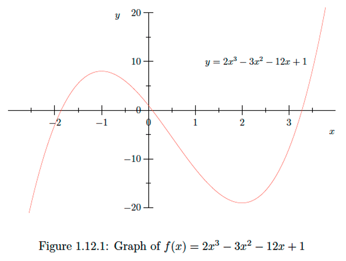
If \(f(x)=2 x^{3}-3 x^{2}-12 x+1,\) then

\[f^{\prime}(x)=6 x^{2}-6 x-12\] and \[f^{\prime \prime}(x)=12 x-6 .\] Hence \(f^{\prime \prime}(x)<0\) when \(x<\frac{1}{2}\) and \(f^{\prime \prime}(x)>0\) when \(x>\frac{1}{2},\) and so the graph of \(f\) is concave downward on the interval \(\left(-\infty, \frac{1}{2}\right)\) and concave upward on the interval \(\left(\frac{1}{2}, \infty\right) .\) One may see the distinction between concave downward and concave upward very clearly in the graph of \(f\) shown in Figure \(1.12 .1 .\) We call a point on the graph of a function \(f\) at which the concavity changes, either from upward to downward or from downward to upward, a point of inflection. In the previous example, \(\left(\frac{1}{2},-\frac{11}{2}\right)\) is a point of inflection.

Exercise \(\PageIndex{4}\)

Find the intervals on which the graph of \(f(x)=5 x^{3}-3 x^{5}\) is concave upward and the intervals on which the graph is concave downward. What are the points of inflection?

Answer

Concave upward on \((-\infty,-1)\) and \((0,1) ;\) concave downward on \((-1,0)\) and \((1, \infty) ;\) Points of inflection: \((-1,-2),(0,0),(1,2)\)

The Second-Derivative Test

Suppose \(c\) is a stationary point of \(f\) and \(f^{\prime \prime}(c)>0 .\) Then, since \(f^{\prime \prime}\) is the derivative of \(f^{\prime}\) and \(f^{\prime}(c)=0,\) for any infinitesimal \(d x \neq 0\),

\[\frac{f^{\prime}(c+d x)-f^{\prime}(c)}{d x}=\frac{f^{\prime}(c+d x)}{d x}>0 .\] It follows that \(f^{\prime}(c+d x)>0\) when \(d x>0\) and \(f^{\prime}(c+d x)<0\) when \(d x<0\). Hence \(f\) is decreasing to the left of \(c\) and increasing to the right of \(c,\) and so \(f\) has a local minimum at \(c .\) Similarly, if \(f^{\prime \prime}(c)<0\) at a stationary point \(c,\) then \(f\) has a local maximum at \(c .\) This result is the second-derivative test.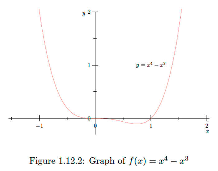

Example \(\PageIndex{5}\)

If \(f(x)=x^{4}-x^{3},\) then

\[f^{\prime}(x)=4 x^{3}-3 x^{2}=x^{2}(4 x-3)\] and \[f^{\prime \prime}(x)=12 x^{2}-6 x=6 x(2 x-1) .\] Hence \(f\) has stationary points \(x=0\) and \(x=\frac{3}{4} .\) Since \[f^{\prime \prime}(0)=0\] and \[f^{\prime \prime}\left(\frac{3}{4}\right)=\frac{9}{4}>0 ,\] we see that \(f\) has a local minimum at \(x=\frac{3}{4} .\) Although the second derivative test tells us nothing about the nature of the critical point \(x=0,\) we know, since \(f\) has a local minimum at \(x=\frac{3}{4},\) that \(f\) is decreasing on \(\left(0, \frac{3}{4}\right)\) and increasing on \(\left(\frac{3}{4}, \infty\right) .\) Moreover, since \(4 x-3<0\) for all \(x<0,\) it follows that \(f^{\prime}(x)<0\) for all \(x<0,\) and so \(f\) is also decreasing on \((-\infty, 0) .\) Hence \(f\) has neither a local maximum nor a local minimum at \(x=0 .\) Finally, since \(f^{\prime \prime}(x)<0\) for \(0<x<\frac{1}{2}\) and \(f^{\prime \prime}(x)>0\) for all other \(x,\) we see that the graph of \(f\) is concave downward on the interval \(\left(0, \frac{1}{2}\right)\) and concave upward on the intervals \((-\infty, 0)\) and \(\left(\frac{1}{2}, \infty\right)\). See Figure \(1.12 .2 .\)

Exercise \(\PageIndex{5}\)

Use the second-derivative test to find all local maximums and minimums of

\[f(x)=x+\frac{1}{x} .\]

Answer

Local maximum of \(-2\) at \(x=-1 ;\) local minimum of 2 at \(x=1\)

Exercise \(\PageIndex{6}\)

Find all local maximums and minimums of \(g(t)=5 t^{7}-7 t^{5}\).

Answer

Local maximum of 2 at \(t=-1 ;\) local minimum of \(-2\) at \(t=1\)