2.5: Applications of Definite Integrals

In this section we will look at several examples of applications for definite integrals.

2.5.1. Area Between Curves

Consider two continuous functions \(f\) and \(g\) on an open interval \(I\) with \(f(x) \leq g(x)\) for all \(x\) in \(I .\) For any \(a<b\) in \(I,\) let \(R(a, b)\) be the region in the plane consisting of the points \((x, y)\) for which \(a \leq x \leq b\) and \(f(x) \leq y \leq g(x)\). That is, \(R(a, b)\) is bounded above by the curve \(y=g(x),\) below by the curve \(y=f(x),\) on the left by the vertical line \(x=a,\) and on the right by the vertical line \(x=b,\) as in Figure \(2.5 .1 .\) Let

\[A(a, b)=\operatorname{area} \text { of } R(a, b).\]

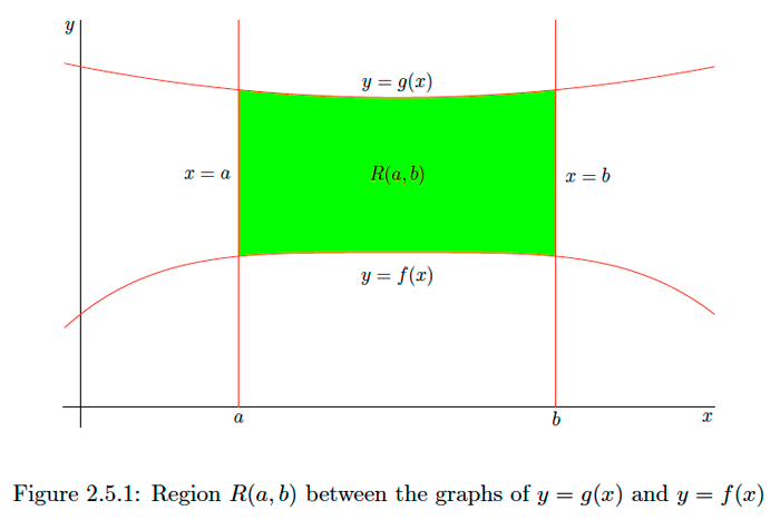
Clearly, for any \(a \leq c \leq b\),

\[A(a, b)=A(a, c)+A(c, b).\] Now for an \(x\) in \(I\) and a positive infinitesimal \(d x,\) let \(c\) be the point at which \(g(u)-f(u)\) attains its minimum value for \(x \leq u \leq x+d x\) and let \(d\) be the point at which \(g(u)-f(u)\) attains its maximum value for \(x \leq u \leq x+d x .\) Then \[(g(c)-f(c)) d x \leq A(x, x+d x) \leq(g(d)-f(d)) d x.\] Moreover, since \[g(c)-f(c) \leq g(x)-f(x) \leq g(d)-f(d),\] we also have \[(g(c)-f(c)) d x \leq(g(x)-f(x)) d x \leq(g(d)-f(d)) d x.\] Putting \((2.5 .3)\) and \((2.5 .5)\) together, we have \[|A(x, d x)-(g(x)-f(x)) d x| \leq((g(d)-f(d))-(f(c)-g(c))) d x\] or \[\frac{|A(x, d x)-(g(x)-f(x)) d x|}{d x} \leq(g(d)-f(d))-(f(c)-g(c))\] Now since \(c \simeq x\) and \(d \simeq x\), \[(g(d)-f(d))-(g(c)-f(c))=(g(d)-g(c))+(f(c)-f(d)) \simeq 0.\]

Hence

\[A(x, d x)-(g(x)-f(x)) d x \sim o(d x).\] It now follows from Theorem 2.4.1 that \[A(a, b)=\int_{a}^{b}(g(x)-f(x)) d x.\]

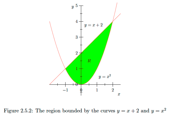
Example \(\PageIndex{1}\)

Let \(A\) be the area of the region \(R\) bounded by the curves with equations \(y=x^{2}\) and \(y=x+2 .\) Note that these curves intersect when \(x^{2}=x+2,\) that is when

\[0=x^{2}-x-2=(x+1)(x-2).\] Hence they intersect at the points \((-1,1)\) and \((2,4),\) and so \(R\) is the region in the plane bounded above by the curve \(y=x+2,\) below by the curve \(y=x^{2},\) on the right by \(x=-1,\) and on the left by \(x=2 .\) See Figure \(2.5 .2 .\) Thus we have \[\begin{aligned} A &=\int_{-1}^{2}\left(x+2-x^{2}\right) d x \\ &=\left.\left(\frac{1}{2} x^{2}+2 x-\frac{1}{3} x^{3}\right)\right|_{-1} ^{2} \\ &=\left(2+4-\frac{8}{3}\right)-\left(\frac{1}{2}-2+\frac{1}{3}\right) \\ &=\frac{9}{2}. \end{aligned}\]

Exercise \(\PageIndex{1}\)

Find the area of the region bounded by the curves \(y=x\) and \(y=x^{2}\).

Answer

\(\frac{1}{6}\)

Exercise \(\PageIndex{2}\)

Find the area of the region bounded by the curves \(y=x^{2}\) and \(y=2-x^{2}\).

Answer

\(\frac{8}{3}\)

Exercise \(\PageIndex{3}\)

Find the area of the region bounded by the curves \(y=\sqrt{x}\) and \(y=x\).

Answer

\(\frac{1}{6}\)

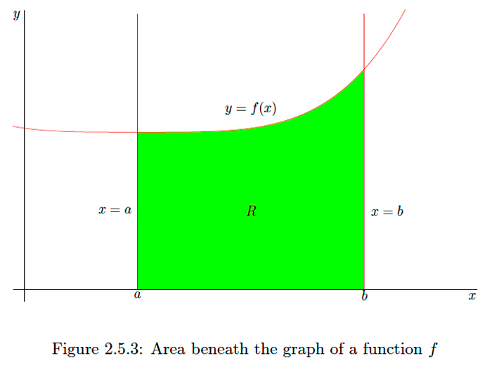
Now consider a continuous function \(f\) on an interval \([a, b]\) with \(f(x) \geq 0\) for all \(x\) in \([a, b] .\) If \(A\) is the area of the region \(R\) bounded above by the graph of \(y=f(x),\) below by the graph of \(y=0\) (that is, the \(x\) -axis), on the right by the vertical line \(x=a \text { , and on the left by the graph of } x=b \text { (see Figure } 2.5 .3),\) then

\[A=\int_{a}^{b}(f(x)-0) d x=\int_{a}^{b} f(x) d x.\] This gives us a geometric interpretation for a the definite integral of a nonnegative function \(f\) over an interval \([a, b]\) as the area beneath the graph of \(f\) and above the \(x\)-axis. the \(x\) axis, then \[A=\int_{a}^{b}(0-f(x)) d x=-\int_{a}^{b} f(x) d x.\] That is, the definite integral of a non-positive function \(f\) over an interval \([a, b]\) is the negative of the area above the graph of \(f\) and beneath the \(x\)-axis. In general, given a continuous function \(f\) on an interval let \(R\) be the region bounded by the \(x\) -axis and the graph of \(y=f(x) .\) If \(A^{+}\) is the area of the part of \(R\) which lies above the \(x\) -axis and \(A^{-}\) is the area of the part of \(R\) which lies below the \(x\)-axis, then \[\int_{a}^{b} f(x) d x=A^{+}-A^{-}.\]

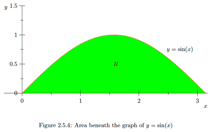
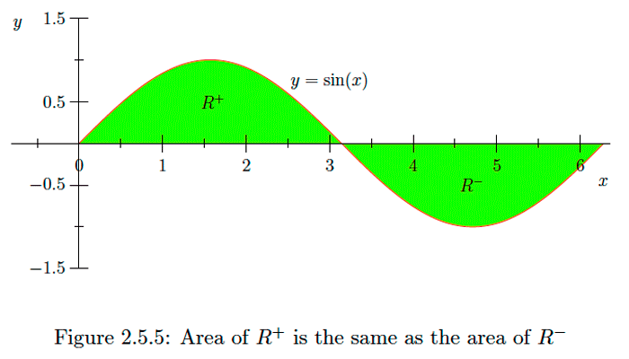
Example \(\PageIndex{3}\)

Note that

\[\int_{0}^{2 \pi} \sin (x) d x=-\left.\cos (x)\right|_{0} ^{2 \pi}=-1+1=0.\] Geometrically, we can see this result in Figure \(2.5 .5 .\) If \(R^{+}\) is the the region beneath the graph of \(y=\sin (x)\) over the interval \([0, \pi]\) and \(R^{-}\) is the region above the graph of \(y=\sin (x)\) over the interval \([0,2 \pi],\) then these two regions have the same area. Hence the integral, which is the area of \(R^{+}\) minus the area of \(R^{-},\) is \(0 .\)

Exercise \(\PageIndex{4}\)

Evaluate

\[\int_{-1}^{1} x^{3} d x \nonumber\]

and explain the result geometrically.

Answer

0

Exercise \(\PageIndex{5}\)

Evaluate

\[\int_{-1}^{2} x d x\] and explain the result geometrically.

Answer

\(\frac{3}{2}\)

Exercise \(\PageIndex{6}\)

Explain, geometrically, why

\[\int_{-1}^{1} \sqrt{1-x^{2}} d x=\frac{\pi}{2}.\]

2.5.2 Volumes

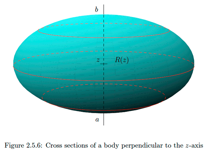
Consider a three-dimensional body \(B\). Given a line, which we will call the \(z\)-axis, let \(V(a, b)\) be the volume of \(B\) which lies between planes which are perpendicular to the \(z\)-axis and pass through \(z=a\) and \(z=b .\) Clearly, for any \(a<c<b\),

\[V(a, b)=V(a, c)+V(c, b).\] Now suppose that, for any \(a \leq x \leq b, R(z)\) is a cross section of \(B\) perpendicular to the \(z\) -axis. See Figure \(2.5 .6 .\) Let \(A(z)\) be the area of \(R(z) .\) We assume \(A\) is a continuous function of \(z .\) For a positive infinitesimal \(d z,\) let \(A\) have, on the interval \([z, z+d z],\) a minimum value at \(c\) and a maximum value at \(d .\) Then \[A(c) d z \leq V(z, z+d z) \leq A(d) d z.\] Since we also have \(A(c) \leq A(z) \leq A(d),\) it follows that \[|V(z, z+d z)-A(z) d z| \leq(A(d)-A(c)) d z.\] Thus \[\frac{|V(z, z+d z)-A(z) d z|}{d z} \leq A(d)-A(c).\] Since \(A\) is continuous and \(d \simeq z\) and \(c \simeq z, A(d)-A(c)\) is infinitesimal. Hence \[V(z, z+d z)-A(z) d z \sim o(d z),\] from which it follows, by Theorem 2.4.1, that \[V(a, b)=\int_{a}^{b} A(z) d z.\]

Example \(\PageIndex{4}\)

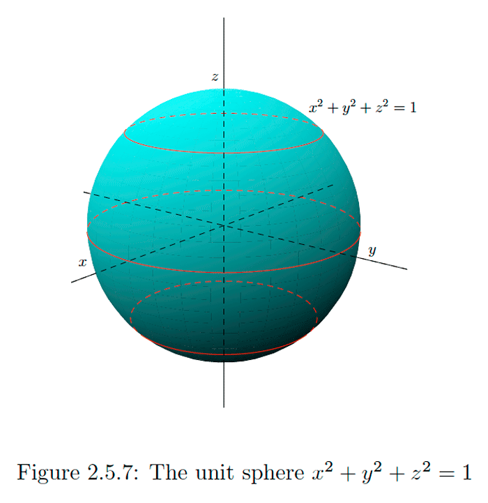
The unit sphere \(S,\) with center at the origin, is the set of all points \(\left.(x, y, z) \text { satisfying } x^{2}+y^{2}+z^{2}=1 \text { (see Figure } 2.5 .7\right) .\) For a fixed value of \(z\) between \(-1\) and \(1,\) the cross section \(R(z)\) of \(S\) perpendicular to the \(z\)-axis is the set of points \((x, y)\) satisfying the equation \(x^{2}+y^{2}=1-z^{2} .\) That is, \(R(z)\) is a circle with radius \(\sqrt{1-z^{2}} .\) Hence \(R(z)\) has area

\[A(z)=\pi\left(1-z^{2}\right).\] If \(V\) is the volume of \(S,\) it now follows that \[\begin{aligned} V &=\int_{-1}^{1} \pi\left(1-z^{2}\right) d x \\ &=\left.\pi\left(z-\frac{1}{3} z^{3}\right)\right|_{-1} ^{1} \\ &=\pi\left(\frac{2}{3}+\frac{2}{3}\right) \\ &=\frac{4 \pi}{3}. \end{aligned}\]

Exercise \(\PageIndex{7}\)

For \(r>0,\) the equation of a sphere \(S\) of radius \(r\) is \(x^{2}+y^{2}+z^{2}=r^{2} .\) Show that the volume of \(S\) is \(\frac{4}{3} \pi r^{3}\).

Exercise \(\PageIndex{8}\)

Let \(P\) be a pyramid with a square base having corners at \((1,1,0),(1,-1,0),(-1,-1,0),\) and \((-1,1,0)\) in the \(x y\) -plane and top vertex at \((0,0,1)\) on the \(z\) -axis. Show that the volume of \(P\) is \(\frac{4}{3} .\)

Example \(\PageIndex{5}\)

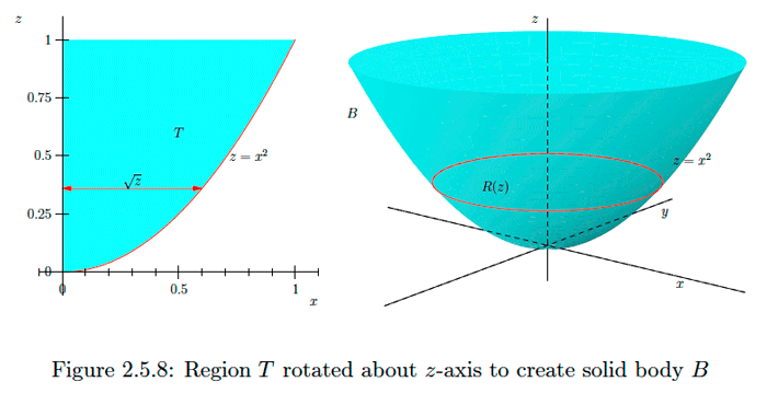
Let \(T\) be the region bounded by the \(z\)-axis and the graph of \(z=x^{2}\) for \(0 \leq x \leq 1 .\) Let \(B\) be three-dimensional body created by rotating \(T\) about the \(z\)-axis. See Figure \(2.5.8.\) If \(R(z)\) is a cross section of \(B\) perpendicular to the \(z\) -axis, then \(R(z)\) is a circle with radius \(\sqrt{z} .\) Thus, if \(A(z)\) is the area of \(R(z),\) we have

\[A(z)=\pi z.\] If \(V\) is the volume of \(B,\) then \[V=\int_{0}^{1} \pi z d z=\left.\pi \frac{z^{2}}{2}\right|_{0} ^{1}=\frac{\pi}{2}.\]

Exercise \(\PageIndex{9}\)

Let \(T\) be the region bounded by \(z\)-axis and the graph of \(z=x\) for \(0 \leq x \leq 2 .\) Find the volume of the solid \(B\) obtained by rotating \(T\) about the \(z\)-axis.

Exercise \(\PageIndex{10}\)

Let \(T\) be the region bounded by \(z\)-axis and the graph of \(z=x^{4}\) for \(0 \leq x \leq 1 .\) Find the volume of the solid \(B\) obtained by rotating \(T\) about the \(z\)-axis.

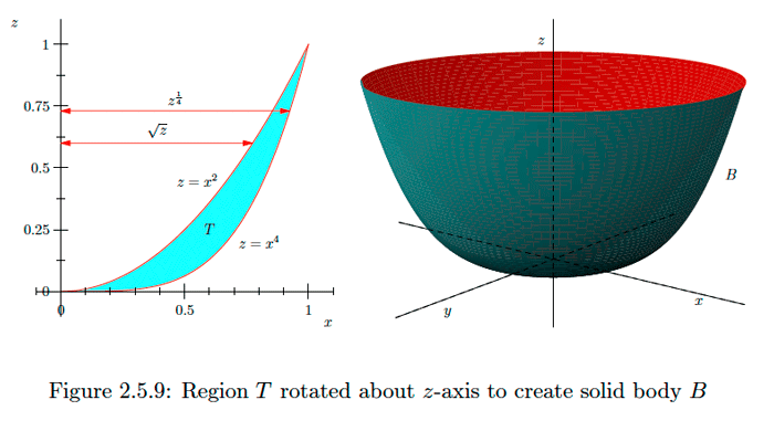
Example \(\PageIndex{6}\)

Let \(T\) be the region bounded by the graphs of \(z=x^{4}\) and \(x=x^{2}\) for \(0 \leq x \leq 1 .\) Let \(B\) be the three-dimensional body created by rotating \(T\) about the \(z\)-axis. See Figure \(2.5 .9 .\) If \(R(z)\) is a cross section of \(B\) perpendicular to the \(z\)-axis, then \(R(z)\) is the region between the circles with radii \(z^{\frac{1}{4}}\) and \(\sqrt{z}\), an annulus. Hence if \(A(z)\) is the area of \(R(z),\) then

\[A(z)=\pi\left(z^{\frac{1}{4}}\right)^{2}-\pi(\sqrt{z})^{2}=\pi(\sqrt{z}-z).\] If \(V\) is the volume of \(B,\) then \[V=\int_{0}^{1} \pi(\sqrt{z}-z) d z=\left.\pi\left(\frac{2}{3} z^{\frac{3}{2}}-\frac{1}{2} z^{2}\right)\right|_{0} ^{1}=\pi\left(\frac{2}{3}-\frac{1}{2}\right)=\frac{\pi}{6}.\]

Exercise \(\PageIndex{11}\)

Let \(T\) be the region bounded by the curves \(z=x\) and \(z=x^{2} .\) Find the volume of the solid \(B\) obtained by rotating \(T\) about the \(z\)-axis.

Answer

\(\frac{\pi}{6}\)

2.5.3 Arc Length

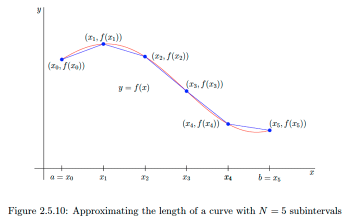
Consider a function \(f\) which is continuolus on the closed interval \([a, b] .\) Let \(C\) be the graph of \(f\) over \([a, b]\) and let \(L\) be the length of \(C .\) To approximate \(L,\) we first divide \([a, b]\) into \(N\) equal subintervals, each of length

\[\Delta x=\frac{b-a}{N},\] and let \(x_{0}=a, x_{1}, x_{2}, \ldots, x_{N}=b\) be the endpoints of the subintervals. If \(L_{i}\) is the length of the line from \(\left(x_{i-1}, f\left(x_{i-1}\right)\right)\) to \(\left(x_{i}, f\left(x_{i}\right)\right),\) for \(i=1,2, \ldots, N\) (see Figure \(2.5 .10),\) then \[L \approx L_{1}+L_{2}+\cdots+L_{N}=\sum_{i=1}^{N} L_{i}.\] Since \[L_{i}=\sqrt{\left(x_{i}-x_{i-1}\right)^{2}+\left(f\left(x_{i}\right)-f\left(x_{i-1}\right)^{2}\right.}=\sqrt{(\Delta x)^{2}+\left(\Delta y_{i}\right)^{2}},\] where \[\Delta y_{i}=f\left(x_{i}\right)-f\left(x_{i-1}\right)=f\left(x_{i-1}+\Delta x\right)-f\left(x_{i-1}\right),\] we have \[L \approx \sum_{i=1}^{N} \sqrt{(\Delta x)^{2}+\left(\Delta y_{i}\right)^{2}}=\sum_{i=1}^{N} \sqrt{1+\left(\frac{\Delta y_{i}}{\Delta x}\right)^{2}} \Delta x.\]

Now we should expect the approximation in \((2.5 .24)\) to become exact when \(N\) is infinite. That is, for \(N\) a positive infinite integer, let

\[d x=\frac{b-a}{N},\] and \[d y=f(x+d x)-f(x).\] If the shadow of \[\sum_{i=1}^{N} \sqrt{1+\left(\frac{d y}{d x}\right)^{2}} d x.\] is the same for any choice of \(N,\) then we call \((2.5 .27)\) the arc length of \(C .\) Now if \(f\) is differentiable on an open interval containing \([a, b],\) and \(f^{\prime}\) is continuous on \([a, b],\) then \((2.5 .27)\) becomes the definite integral of \(\sqrt{1+\left(f^{\prime}(x)\right)^{2}} .\) That is, the arc length of \(C\) is given by \[L=\int_{a}^{b} \sqrt{1+\left(f^{\prime}(x)\right)^{2}} d x.\]

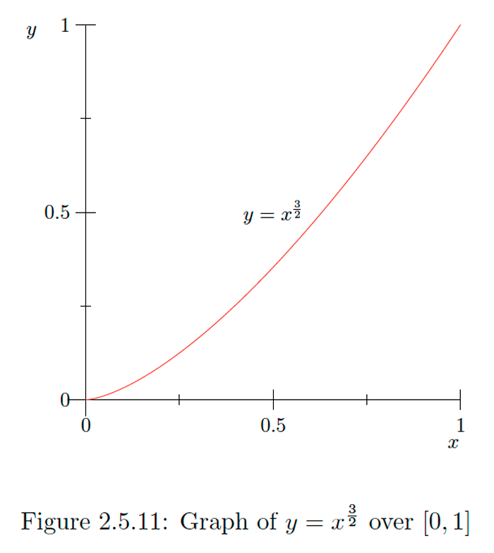
Example \(\PageIndex{7}\)

Let \(C\) be the graph of \(f(x)=x^{\frac{3}{2}}\) over the interval \([0,1]\) (see Figure \(2.5 .11)\) and let \(L\) be the length of \(C .\) since \(f^{\prime}(x)=\frac{3}{2} \sqrt{x},\) we have

\[L=\int_{0}^{1} \sqrt{1+\frac{9}{4} x} d x.\] Now \[\int \sqrt{x} d x=\frac{2}{3} x^{\frac{3}{2}}+c,\] so we might expect an integral of \(\sqrt{1+\frac{9}{4}}\) to be \[\frac{2}{3}\left(1+\frac{9}{4} x\right)^{\frac{3}{2}}+c.\] However, \[\frac{d}{d x} \frac{2}{3}\left(1+\frac{9}{4} x\right)^{\frac{3}{2}}=\frac{9}{4} \sqrt{1+\frac{9}{4} x},\] and so, dividing our original guess by \(\frac{9}{4},\) we have \[\int \sqrt{1+\frac{9}{4}} x d x=\frac{8}{27}\left(1+\frac{9}{4} x\right)^{\frac{3}{2}}+c,\] which may be verified by differentiation. Hence \[\begin{aligned} L &=\int_{0}^{1} \sqrt{1+\frac{9}{4} x} d x \\ &=\left.\frac{8}{27}\left(1+\frac{9}{4} x\right)^{\frac{3}{2}}\right|_{0} ^{1} \\ &=\frac{8}{27}\left(\frac{13 \sqrt{13}}{8}-1\right) \\ &=\frac{13 \sqrt{13}-8}{27} \\ & \approx 1.4397. \end{aligned}\]

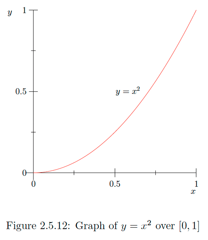
Example \(\PageIndex{8}\)

Let \(C\) be the graph of \(f(x)=x^{2}\) over the interval \([0,1]\) (see Figure 2.5 .12 ) and let \(L\) be the length of \(C .\) since \(f^{\prime}(x)=2 x\),

\[L=\int_{0}^{1} \sqrt{1+4 x^{2}} d x.\] However, we do not have the tools at this time to evaluate this definite integral exactly. Still, we may use \((2.5 .24)\) to find an approximation for \(L .\) For example, if we take \(N=100\) in \((2.5 .24),\) then \(\Delta x=0.01\) and \[\begin{aligned} \Delta y_{i} &=f(0.01 i)-f(0.01(i-1)) \\ &=(0.01 i)^{2}-(0.01(i-1))^{2} \\ &=0.0001\left(i^{2}-\left(i^{2}-2 i+1\right)\right) \\ &=0.0001(2 i-1) \end{aligned}\] for \(i=1,2, \ldots, N,\) and so \[L \approx \sum_{i=1}^{100} \sqrt{(\Delta x)^{2}+\left(\Delta y_{i}\right)^{2}} \approx 1.4789.\] We will return to this example in Examples 2.6.19 and 2.7.9 to find an exact expression for \(L .\)

Exercise \(\PageIndex{12}\)

Let \(C\) be the graph of \(y=\frac{2}{3} x^{\frac{3}{2}}\) over the interval \([1,3] .\) Find the length of \(C\).

Answer

\(\frac{16-4 \sqrt{2}}{3}\)

Exercise \(\PageIndex{13}\)

Let \(C\) be the graph of \(y=\sin (x)\) over the interval \([0, \pi]\). Use \((2.5 .24)\) with \(N=10\) to approximate the length of \(C .\)

Answer

3.8153