7.1: Two Examples

Up to now we have been concerned with extracting information about how a function changes from the function itself. Given knowledge about an object's position, for example, we want to know the object's speed. Given information about the height of a curve we want to know its slope. We now consider problems that are, whether obviously or not, the reverse of such problems.

So for $t=1$, at least, this rather cumbersome approach gives the same answer as the first approach. But really there's nothing special about $t=1$; let's just call it $t$ instead. In this case the approximate distance traveled during time interval number $i$ is $3(i-1)(t/n)(t/n)=3(i-1)t^2/n^2$, that is, speed $3(i-1)(t/n)$ times time $t/n$, and the total distance traveled is approximately $$(0){t\over n}+3(1){t^2\over n^2}+3(2){t^2\over n^2}+ 3(3){t^2\over n^2}+\cdots+3(n-1){t^2\over n^2}.$$ As before we can simplify this to $${3t^2\over n^2}(0+1+2+\cdots+(n-1))={3t^2\over n^2}{n^2-n\over2}= {3\over2}t^2\left(1-{1\over n}\right).$$ In the limit, as $n$ gets larger, this gets closer and closer to $(3/2)t^2$ and the approximated position of the object gets closer and closer to $(3/2)t^2+10$, so the actual position is $(3/2)t^2+10$, exactly the answer given by the first approach to the problem.

There is here no obvious analogue to the first approach in the previous example, but the second approach works fine. (Because the function $y=3x$ is so simple, there is another approach that works here, but it is even more limited in potential application than is approach number one.) How might we approximate the desired area? We know how to compute areas of rectangles, so we approximate the area by rectangles. Jumping straight to the general case, suppose we divide the interval between 0 and $x$ into $n$ equal subintervals, and use a rectangle above each subinterval to approximate the area under the curve. There are many ways we might do this, but let's use the height of the curve at the left endpoint of the subinterval as the height of the rectangle, as in figure 7.1.1. The height of rectangle number $i$ is then $3(i-1)(x/n)$, the width is $x/n$, and the area is \ 3(i-1)(x^2/n^2)\. The total area of the rectangles is $$(0){x\over n}+3(1){x^2\over n^2}+3(2){x^2\over n^2}+ 3(3){x^2\over n^2}+\cdots+3(n-1){x^2\over n^2}.$$ By factoring out $3x^2/n^2$ this simplifies to $${3x^2\over n^2}(0+1+2+\cdots+(n-1))={3x^2\over n^2}{n^2-n\over2}= {3\over2}x^2\left(1-{1\over n}\right).$$ As $n$ gets larger this gets closer and closer to $3x^2/2$, which must therefore be the true area under the curve.

Figure 7.1.1. Approximating the area under $y=3x$ with rectangles.

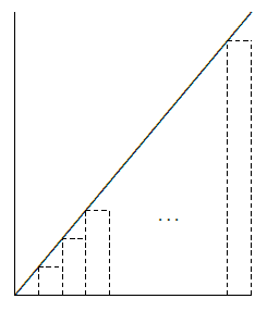
What you will have noticed, of course, is that while the problem in the second example appears to be much different than the problem in the first example, and while the easy approach to problem one does not appear to apply to problem two, the "approximation'' approach works in both, and moreover the {\it calculations are identical.} As we will see, there are many, many problems that appear much different on the surface but that turn out to be the same as these problems, in the sense that when we try to approximate solutions we end up with mathematics that looks like the two examples, though of course the function involved will not always be so simple.
Even better, we now see that while the second problem did not appear to be amenable to approach one, it can in fact be solved in the same way. The reasoning is this: we know that problem one can be solved easily by finding a function whose derivative is $3t$. We also know that mathematically the two problems are the same, because both can be solved by taking a limit of a sum, and the sums are identical. Therefore, we don't really need to compute the limit of either sum because we know that we will get the same answer by computing a function with the derivative $3t$ or, which is the same thing, $3x$.

It's true that the first problem had the added complication of the "10'', and we certainly need to be able to deal with such minor variations, but that turns out to be quite simple. The lesson then is this: whenever we can solve a problem by taking the limit of a sum of a certain form, we can instead of computing the (often nasty) limit find a new function with a certain derivative.

Contributors

David Guichard (Whitman College)

• Integrated by Justin Marshall.