8.7: Numerical Integration

We have now seen some of the most generally useful methods for discovering antiderivatives, and there are others. Unfortunately, some functions have no simple antiderivatives; in such cases if the value of a definite integral is needed it will have to be approximated. We will see two methods that work reasonably well and yet are fairly simple; in some cases more sophisticated techniques will be needed.

Of course, we already know one way to approximate an integral: if we think of the integral as computing an area, we can add up the areas of some rectangles. While this is quite simple, it is usually the case that a large number of rectangles is needed to get acceptable accuracy. A similar approach is much better: we approximate the area under a curve over a small interval as the area of a trapezoid. In figure 8.6.1 we see an area under a curve approximated by rectangles and by trapezoids; it is apparent that the trapezoids give a substantially better approximation on each subinterval.

Figure 8.6.1. Approximating an area with rectangles and with trapezoids.

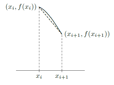
As with rectangles, we divide the interval into \(n\) equal subintervals of length \(\Delta x\). A typical trapezoid is pictured in figure 8.6.2; it has area \( {f(x_i)+f(x_{i+1})\over2}\Delta x\). If we add up the areas of all trapezoids we get

\[ \eqalign{ {f(x_0)+f(x_1)\over2}\Delta x&+{f(x_1)+f(x_2)\over2}\Delta x+\cdots+ {f(x_{n-1})+f(x_n)\over2}\Delta x=\cr &\left({f(x_0)\over2}+f(x_1)+f(x_2)+\cdots+f(x_{n-1})+{f(x_n)\over2}\right) \Delta x.\cr} \]

This is usually known as the Trapezoid Rule. For a modest number of subintervals this is not too difficult to do with a calculator; a computer can easily do many subintervals.

Figure 8.6.2. A single trapezoid.

In practice, an approximation is useful only if we know how accurate it is; for example, we might need a particular value accurate to three decimal places. When we compute a particular approximation to an integral, the error is the difference between the approximation and the true value of the integral. For any approximation technique, we need an error estimate, a value that is guaranteed to be larger than the actual error. If \(A\) is an approximation and \(E\) is the associated error estimate, then we know that the true value of the integral is between \(A-E\) and \(A+E\). In the case of our approximation of the integral, we want \(E=E(\Delta x)\) to be a function of \(\Delta x\) that gets small rapidly as \(\Delta x\) gets small. Fortunately, for many functions, there is such an error estimate associated with the trapezoid approximation.

Theorem 8.6.1: The Trapezoid Approximation

Suppose \(f\) has a second derivative \(f''\) everywhere on the interval \([a,b]\), and \(|f''(x)|\le M\) for all \(x\) in the interval. With \(\Delta x= (b-a)/n\), an error estimate for the trapezoid approximation is

\[ E(\Delta x) = {b-a\over12}M(\Delta x)^2={(b-a)^3\over 12n^2}M. \]

Let's see how we can use this.

Had we immediately tried \(n=13\) this would have given us the desired answer.

The trapezoid approximation works well, especially compared to rectangles, because the tops of the trapezoids form a reasonably good approximation to the curve when \(\Delta x\) is fairly small. We can extend this idea: what if we try to approximate the curve more closely, by using something other than a straight line? The obvious candidate is a parabola: if we can approximate a short piece of the curve with a parabola with equation \( y=ax^2+bx+c\), we can easily compute the area under the parabola.

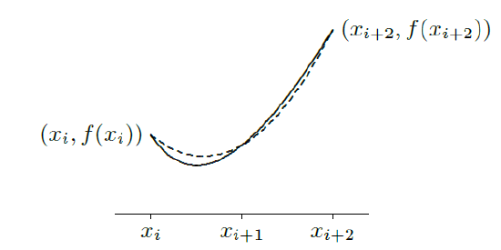
There are an infinite number of parabolas through any two given points, but only one through three given points. If we find a parabola through three consecutive points \((x_i,f(x_i))\), \((x_{i+1},f(x_{i+1}))\), \((x_{i+2},f(x_{i+2}))\) on the curve, it should be quite close to the curve over the whole interval \([x_i,x_{i+2}]\), as in figure 8.6.3. If we divide the interval \([a,b]\) into an even number of subintervals, we can then approximate the curve by a sequence of parabolas, each covering two of the subintervals.

For this to be practical, we would like a simple formula for the area under one parabola, namely, the parabola through \((x_i,f(x_i))\), \((x_{i+1},f(x_{i+1}))\), and \((x_{i+2},f(x_{i+2}))\). That is, we should attempt to write down the parabola \(y=ax^2+bx+c\) through these points and then integrate it, and hope that the result is fairly simple. Although the algebra involved is messy, this turns out to be possible. The algebra is well within the capability of a good computer algebra system like Sage, so we will present the result without all of the algebra; you can see how to do it in this Sage worksheet.

To find the parabola, we solve these three equations for \(a\), \(b\), and \(c\):

\[ \eqalign{ f(x_i)&=a(x_{i+1}-\Delta x)^2+b(x_{i+1}-\Delta x)+c\cr f(x_{i+1})&=a(x_{i+1})^2+b(x_{i+1})+c\cr f(x_{i+2})&=a(x_{i+1}+\Delta x)^2+b(x_{i+1}+\Delta x)+c\cr} \]

Not surprisingly, the solutions turn out to be quite messy. Nevertheless, Sage can easily compute and simplify the integral to get

\[ \int_{x_{i+1}-\Delta x}^{x_{i+1}+\Delta x} ax^2+bx+c\,dx= {\Delta x\over3}(f(x_i)+4f(x_{i+1})+f(x_{i+2})). \]

Now the sum of the areas under all parabolas is

\[ \displaylines{ {\Delta x\over3}(f(x_0)+4f(x_{1})+f(x_{2})+f(x_2)+4f(x_{3})+f(x_{4})+\cdots +f(x_{n-2})+4f(x_{n-1})+f(x_{n}))=\cr {\Delta x\over3}(f(x_0)+4f(x_{1})+2f(x_{2})+4f(x_{3})+2f(x_{4})+\cdots +2f(x_{n-2})+4f(x_{n-1})+f(x_{n})).\cr} \]

This is just slightly more complicated than the formula for trapezoids; we need to remember the alternating 2 and 4 coefficients. This approximation technique is referred to as Simpson's Rule.

Figure 8.6.3. A parabola (dashed) approximating a curve (solid).

As with the trapezoid method, this is useful only with an error estimate:

Theorem 8.6.3: Simpson Approximation Error

Suppose \(f\) has a fourth derivative \(f^{(4)}\) everywhere on the interval \([a,b]\), and \(|f^{(4)}(x)|\le M\) for all \(x\) in the interval. With \(\Delta x= (b-a)/n\), an error estimate for Simpson's approximation is

\[ E(\Delta x) = {b-a\over180}M(\Delta x)^4={(b-a)^5\over 180n^4}M. \]

So the true value of the integral is between \(0.746855-0.0003=0.746555\) and \(0.746855+0.0003=0.7471555\), both of which round to \(0.75\).

Contributors

David Guichard (Whitman College)

• Integrated by Justin Marshall.