12.1: The Coordinate System
- Page ID
- 922
\( \newcommand{\vecs}[1]{\overset { \scriptstyle \rightharpoonup} {\mathbf{#1}} } \)
\( \newcommand{\vecd}[1]{\overset{-\!-\!\rightharpoonup}{\vphantom{a}\smash {#1}}} \)
\( \newcommand{\dsum}{\displaystyle\sum\limits} \)
\( \newcommand{\dint}{\displaystyle\int\limits} \)
\( \newcommand{\dlim}{\displaystyle\lim\limits} \)
\( \newcommand{\id}{\mathrm{id}}\) \( \newcommand{\Span}{\mathrm{span}}\)
( \newcommand{\kernel}{\mathrm{null}\,}\) \( \newcommand{\range}{\mathrm{range}\,}\)
\( \newcommand{\RealPart}{\mathrm{Re}}\) \( \newcommand{\ImaginaryPart}{\mathrm{Im}}\)
\( \newcommand{\Argument}{\mathrm{Arg}}\) \( \newcommand{\norm}[1]{\| #1 \|}\)
\( \newcommand{\inner}[2]{\langle #1, #2 \rangle}\)
\( \newcommand{\Span}{\mathrm{span}}\)
\( \newcommand{\id}{\mathrm{id}}\)
\( \newcommand{\Span}{\mathrm{span}}\)
\( \newcommand{\kernel}{\mathrm{null}\,}\)
\( \newcommand{\range}{\mathrm{range}\,}\)
\( \newcommand{\RealPart}{\mathrm{Re}}\)
\( \newcommand{\ImaginaryPart}{\mathrm{Im}}\)
\( \newcommand{\Argument}{\mathrm{Arg}}\)
\( \newcommand{\norm}[1]{\| #1 \|}\)
\( \newcommand{\inner}[2]{\langle #1, #2 \rangle}\)
\( \newcommand{\Span}{\mathrm{span}}\) \( \newcommand{\AA}{\unicode[.8,0]{x212B}}\)
\( \newcommand{\vectorA}[1]{\vec{#1}} % arrow\)
\( \newcommand{\vectorAt}[1]{\vec{\text{#1}}} % arrow\)
\( \newcommand{\vectorB}[1]{\overset { \scriptstyle \rightharpoonup} {\mathbf{#1}} } \)
\( \newcommand{\vectorC}[1]{\textbf{#1}} \)
\( \newcommand{\vectorD}[1]{\overrightarrow{#1}} \)
\( \newcommand{\vectorDt}[1]{\overrightarrow{\text{#1}}} \)
\( \newcommand{\vectE}[1]{\overset{-\!-\!\rightharpoonup}{\vphantom{a}\smash{\mathbf {#1}}}} \)
\( \newcommand{\vecs}[1]{\overset { \scriptstyle \rightharpoonup} {\mathbf{#1}} } \)
\(\newcommand{\longvect}{\overrightarrow}\)
\( \newcommand{\vecd}[1]{\overset{-\!-\!\rightharpoonup}{\vphantom{a}\smash {#1}}} \)
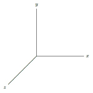
\(\newcommand{\avec}{\mathbf a}\) \(\newcommand{\bvec}{\mathbf b}\) \(\newcommand{\cvec}{\mathbf c}\) \(\newcommand{\dvec}{\mathbf d}\) \(\newcommand{\dtil}{\widetilde{\mathbf d}}\) \(\newcommand{\evec}{\mathbf e}\) \(\newcommand{\fvec}{\mathbf f}\) \(\newcommand{\nvec}{\mathbf n}\) \(\newcommand{\pvec}{\mathbf p}\) \(\newcommand{\qvec}{\mathbf q}\) \(\newcommand{\svec}{\mathbf s}\) \(\newcommand{\tvec}{\mathbf t}\) \(\newcommand{\uvec}{\mathbf u}\) \(\newcommand{\vvec}{\mathbf v}\) \(\newcommand{\wvec}{\mathbf w}\) \(\newcommand{\xvec}{\mathbf x}\) \(\newcommand{\yvec}{\mathbf y}\) \(\newcommand{\zvec}{\mathbf z}\) \(\newcommand{\rvec}{\mathbf r}\) \(\newcommand{\mvec}{\mathbf m}\) \(\newcommand{\zerovec}{\mathbf 0}\) \(\newcommand{\onevec}{\mathbf 1}\) \(\newcommand{\real}{\mathbb R}\) \(\newcommand{\twovec}[2]{\left[\begin{array}{r}#1 \\ #2 \end{array}\right]}\) \(\newcommand{\ctwovec}[2]{\left[\begin{array}{c}#1 \\ #2 \end{array}\right]}\) \(\newcommand{\threevec}[3]{\left[\begin{array}{r}#1 \\ #2 \\ #3 \end{array}\right]}\) \(\newcommand{\cthreevec}[3]{\left[\begin{array}{c}#1 \\ #2 \\ #3 \end{array}\right]}\) \(\newcommand{\fourvec}[4]{\left[\begin{array}{r}#1 \\ #2 \\ #3 \\ #4 \end{array}\right]}\) \(\newcommand{\cfourvec}[4]{\left[\begin{array}{c}#1 \\ #2 \\ #3 \\ #4 \end{array}\right]}\) \(\newcommand{\fivevec}[5]{\left[\begin{array}{r}#1 \\ #2 \\ #3 \\ #4 \\ #5 \\ \end{array}\right]}\) \(\newcommand{\cfivevec}[5]{\left[\begin{array}{c}#1 \\ #2 \\ #3 \\ #4 \\ #5 \\ \end{array}\right]}\) \(\newcommand{\mattwo}[4]{\left[\begin{array}{rr}#1 \amp #2 \\ #3 \amp #4 \\ \end{array}\right]}\) \(\newcommand{\laspan}[1]{\text{Span}\{#1\}}\) \(\newcommand{\bcal}{\cal B}\) \(\newcommand{\ccal}{\cal C}\) \(\newcommand{\scal}{\cal S}\) \(\newcommand{\wcal}{\cal W}\) \(\newcommand{\ecal}{\cal E}\) \(\newcommand{\coords}[2]{\left\{#1\right\}_{#2}}\) \(\newcommand{\gray}[1]{\color{gray}{#1}}\) \(\newcommand{\lgray}[1]{\color{lightgray}{#1}}\) \(\newcommand{\rank}{\operatorname{rank}}\) \(\newcommand{\row}{\text{Row}}\) \(\newcommand{\col}{\text{Col}}\) \(\renewcommand{\row}{\text{Row}}\) \(\newcommand{\nul}{\text{Nul}}\) \(\newcommand{\var}{\text{Var}}\) \(\newcommand{\corr}{\text{corr}}\) \(\newcommand{\len}[1]{\left|#1\right|}\) \(\newcommand{\bbar}{\overline{\bvec}}\) \(\newcommand{\bhat}{\widehat{\bvec}}\) \(\newcommand{\bperp}{\bvec^\perp}\) \(\newcommand{\xhat}{\widehat{\xvec}}\) \(\newcommand{\vhat}{\widehat{\vvec}}\) \(\newcommand{\uhat}{\widehat{\uvec}}\) \(\newcommand{\what}{\widehat{\wvec}}\) \(\newcommand{\Sighat}{\widehat{\Sigma}}\) \(\newcommand{\lt}{<}\) \(\newcommand{\gt}{>}\) \(\newcommand{\amp}{&}\) \(\definecolor{fillinmathshade}{gray}{0.9}\)So far we have been investigating functions of the form \(y=f(x)\), with one independent and one dependent variable. Such functions can be represented in two dimensions, using two numerical axes that allow us to identify every point in the plane with two numbers. We now want to talk about three-dimensional space; to identify every point in three dimensions we require three numerical values. The obvious way to make this association is to add one new axis, perpendicular to the \(x\) and \(y\) axes we already understand. We could, for example, add a third axis, the \(z\) axis, with the positive \(z\) axis coming straight out of the page, and the negative \(z\) axis going out the back of the page. This is difficult to work with on a printed page, so more often we draw a view of the three axes from an angle:

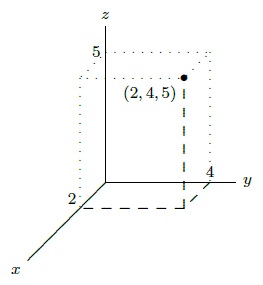
You must then imagine that the \(z\) axis is perpendicular to the other two. Just as we have investigated functions of the form \(y=f(x)\) in two dimensions, we will investigate three dimensions largely by considering functions; now the functions will (typically) have the form \(z=f(x,y)\). Because we are used to having the result of a function graphed in the vertical direction, it is somewhat easier to maintain that convention in three dimensions. To accomplish this, we normally rotate the axes so that \(z\) points up; the result is then:

Note that if you imagine looking down from above, along the \(z\) axis, the positive \(z\) axis will come straight toward you, the positive \(y\) axis will point up, and the positive \(x\) axis will point to your right, as usual. Any point in space is identified by providing the three coordinates of the point, as shown; naturally, we list the coordinates in the order \((x,y,z)\). One useful way to think of this is to use the \(x\) and \(y\) coordinates to identify a point in the \(x\)-\(y\) plane, then move straight up (or down) a distance given by the \(z\) coordinate.
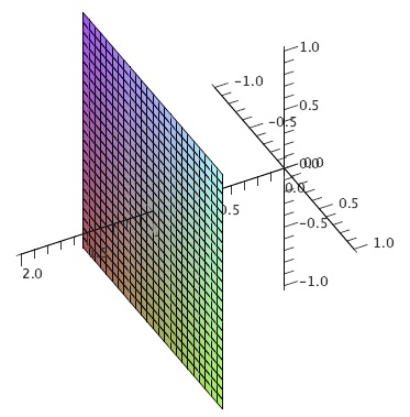
It is now fairly simple to understand some "shapes'' in three dimensions that correspond to simple conditions on the coordinates. In two dimensions the equation \(x=1\) describes the vertical line through \((1,0)\). In three dimensions, it still describes all points with \(x\)-coordinate 1, but this is now a plane, as in Figure 12.1.1.

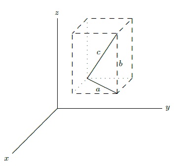
Recall the very useful distance formula in two dimensions: the distance between points \( (x_1,y_1)\) and \( (x_2,y_2)\) is \( \sqrt{(x_1-x_2)^2+(y_1-y_2)^2}\); this comes directly from the Pythagorean theorem. What is the distance between two points \( (x_1,y_1,z_1)\) and \( (x_2,y_2,z_2)\) in three dimensions? Geometrically, we want the length of the long diagonal labeled \(c\) in the "box'' in Figure 12.1.2. Since \(a\), \(b\), \(c\) form a right triangle, \( a^2+b^2=c^2\). \(b\) is the vertical distance between \( (x_1,y_1,z_1)\) and \( (x_2,y_2,z_2)\), so \( b=|z_1-z_2|\). The length \(a\) runs parallel to the \(x-y\) plane, so it is simply the distance between \( (x_1,y_1)\) and \( (x_2,y_2)\), that is, \( a^2=(x_1-x_2)^2+(y_1-y_2)^2\). Now we see that
\[ c^2=(x_1-x_2)^2+(y_1-y_2)^2+(z_1-z_2)^2 \nonumber \]
and
\[ c=\sqrt{(x_1-x_2)^2+(y_1-y_2)^2+(z_1-z_2)^2}. \nonumber \]
It is sometimes useful to give names to points, for example we might let \(P_1=(x_1,y_1,z_1)\), or more concisely we might refer to the point \(P_1(x_1,y_1,z_1)\), and subsequently use just \(P_1\). Distance between two points in either two or three dimensions is sometimes denoted by \(d\), so for example the formula for the distance between \(P_1(x_1,y_1,z_1)\) and \(P_2(x_2,y_2,z_2)\) might be expressed as
\[d(P_1,P_2)=\sqrt{(x_1-x_2)^2+(y_1-y_2)^2+(z_1-z_2)^2}. \nonumber \]

In two dimensions, the distance formula immediately gives us the equation of a circle: the circle of radius \(r\) and center at \((h,k)\) consists of all points \((x,y)\) at distance \(r\) from \((h,k)\), so the equation is \( r=\sqrt{(x-h)^2+(y-k)^2}\) or \( r^2=(x-h)^2+(y-k)^2\). Now we can get the similar equation \( r^2=(x-h)^2+(y-k)^2+(z-l)^2\), which describes all points \((x,y,z)\) at distance \(r\) from \((h,k,l)\), namely, the sphere with radius \(r\) and center \((h,k,l)\).
Contributors
Integrated by Justin Marshall.


