12.2: Vectors

A vector is a quantity consisting of a non-negative magnitude and a direction. We could represent a vector in two dimensions as \((m,\theta)\), where \(m\) is the magnitude and \(\theta\) is the direction, measured as an angle from some agreed upon direction. For example, we might think of the vector \( (5,45^\circ)\) as representing "5 km toward the northeast''; that is, this vector might be a displacement vector, indicating, say, that your grandfather walked 5 kilometers toward the northeast to school in the snow. On the other hand, the same vector could represent a velocity, indicating that your grandfather walked at 5 km/hr toward the northeast. What the vector does not indicate is where this walk occurred: a vector represents a magnitude and a direction, but not a location. Pictorially it is useful to represent a vector as an arrow; the direction of the vector, naturally, is the direction in which the arrow points; the magnitude of the vector is reflected in the length of the arrow.

It turns out that many, many quantities behave as vectors, e.g., displacement, velocity, acceleration, force. Already we can get some idea of their usefulness using displacement vectors. Suppose that your grandfather walked 5 km NE and then 2 km SSE; if the terrain allows, and perhaps armed with a compass, how could your grandfather have walked directly to his destination? We can use vectors (and a bit of geometry) to answer this question. We begin by noting that since vectors do not include a specification of position, we can "place'' them anywhere that is convenient. So we can picture your grandfather's journey as two displacement vectors drawn head to tail:

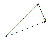
The displacement vector for the shortcut route is the vector drawn with a dashed line, from the tail of the first to the head of the second. With a little trigonometry, we can compute that the third vector has magnitude approximately 4.62 and direction \( 21.43^\circ\), so walking 4.62 km in the direction \( 21.43^\circ\) north of east (approximately ENE) would get your grandfather to school. This sort of calculation is so common, we dignify it with a name: we say that the third vector is the sum of the other two vectors. There is another common way to picture the sum of two vectors. Put the vectors tail to tail and then complete the parallelogram they indicate; the sum of the two vectors is the diagonal of the parallelogram:

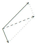
This is a more natural representation in some circumstances. For example, if the two original vectors represent forces acting on an object, the sum of the two vectors is the net or effective force on the object, and it is nice to draw all three with their tails at the location of the object.

We also define scalar multiplication for vectors: if \(\bf A\) is a vector \((m,\theta)\) and \(a\ge 0\) is a real number, the vector \(a\bf A\) is \((am,\theta)\), namely, it points in the same direction but has \(a\) times the magnitude. If \(a < 0\), \(a\bf A\) is \((|a|m,\theta+\pi)\), with \(|a|\) times the magnitude and pointing in the opposite direction (unless we specify otherwise, angles are measured in radians).

Now we can understand subtraction of vectors: \({\bf A}-{\bf B}={\bf A}+(-1){\bf B}\):

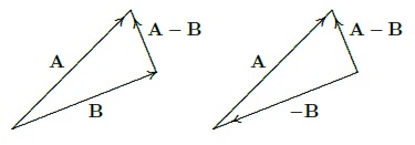
Note that as you would expect, \({\bf B} + ({\bf A}-{\bf B}) = {\bf A}\).

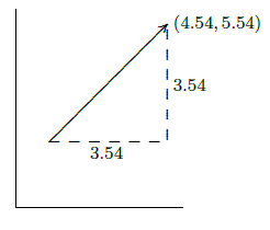
We can represent a vector in ways other than \((m,\theta)\), and in fact \((m,\theta)\) is not generally used at all. How else could we describe a particular vector? Consider again the vector \( (5,45^\circ)\). Let's draw it again, but impose a coordinate system. If we put the tail of the arrow at the origin, the head of the arrow ends up at the point \( (5/\sqrt2,5/\sqrt2)\approx(3.54, 3.54)\).

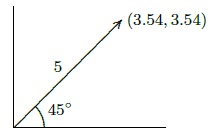
In this picture the coordinates \((3.54,3.54)\) identify the head of the arrow, provided we know that the tail of the arrow has been placed at \((0,0)\). Then in fact the vector can always be identified as \((3.54,3.54)\), no matter where it is placed; we just have to remember that the numbers 3.54 must be interpreted as a change from the position of the tail, not as the actual coordinates of the arrow head; to emphasize this we will write \(\langle 3.54,3.54\rangle\) to mean the vector and \((3.54,3.54)\) to mean the point. Then if the vector \(\langle 3.54,3.54\rangle\) is drawn with its tail at \((1,2)\) it looks like this:

Consider again the two part trip: 5 km NE and then 2 km SSE. The vector representing the first part of the trip is \( \langle 5/\sqrt2,5/\sqrt2\rangle\), and the second part of the trip is represented by \(\langle 2\cos(-3\pi/8),2\sin(-3\pi/8)\rangle \approx\langle 0.77,-1.85 \rangle\). We can represent the sum of these with the usual head to tail picture:

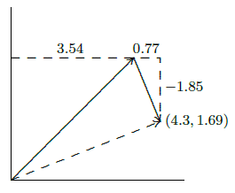
It is clear from the picture that the coordinates of the destination point are \( (5/\sqrt2+2\cos(-3\pi/8),5/\sqrt2+2\sin(-3\pi/8))\) or approximately \((4.3,1.69)\), so the sum of the two vectors is \( \langle 5/\sqrt2+2\cos(-3\pi/8),5/\sqrt2+2\sin(-3\pi/8)\rangle \approx \langle 4.3,1.69\rangle\). Adding the two vectors is easier in this form than in the \((m,\theta)\) form, provided that we're willing to have the answer in this form as well.

It is easy to see that scalar multiplication and vector subtraction are also easy to compute in this form: \(a\langle v,w\rangle=\langle av,aw\rangle\) and \( \langle v_1,w_1\rangle - \langle v_2,w_2\rangle =\langle v_1-v_2,w_1-w_2\rangle\). What about the magnitude? The magnitude of the vector \(\langle v,w\rangle\) is still the length of the corresponding arrow representation; this is the distance from the origin to the point \((v,w)\), namely, the distance from the tail to the head of the arrow. We know how to compute distances, so the magnitude of the vector is simply \( \sqrt{v^2+w^2}\), which we also denote with absolute value bars: \( |\langle v,w\rangle|=\sqrt{v^2+w^2}\).

In three dimensions, vectors are still quantities consisting of a magnitude and a direction, but of course there are many more possible directions. It's not clear how we might represent the direction explicitly, but the coordinate version of vectors makes just as much sense in three dimensions as in two. By \(\langle 1,2,3\rangle\) we mean the vector whose head is at \((1,2,3)\) if its tail is at the origin. As before, we can place the vector anywhere we want; if it has its tail at \((4,5,6)\) then its head is at \((5,7,9)\). It remains true that arithmetic is easy to do with vectors in this form:

\[\eqalign{ &a\langle v_1,v_2,v_3\rangle=\langle av_1,av_2,av_3\rangle\cr &\langle v_1,v_2,v_3\rangle + \langle w_1,w_2,w_3\rangle =\langle v_1+w_1,v_2+w_2,v_3+w_3\rangle\cr &\langle v_1,v_2,v_3\rangle - \langle w_1,w_2,w_3\rangle =\langle v_1-w_1,v_2-w_2,v_3-w_3\rangle\cr} \]

The magnitude of the vector is again the distance from the origin to the head of the arrow, or \( |\langle v_1,v_2,v_3\rangle|=\sqrt{v_1^2+v_2^2+v_3^2}\).

Figure 12.2.1. The vector \(\langle 2,4,5\rangle\) with its tail at the origin.

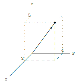
Three particularly simple vectors turn out to be quite useful: \({\bf i}=\langle1,0,0\rangle\), \({\bf j}=\langle0,1,0\rangle\), and \({\bf k}=\langle0,0,1\rangle\). These play much the same role for vectors that the axes play for points. In particular, notice that

\[\eqalign{ \langle v_1,v_2,v_3\rangle &= \langle v_1,0,0\rangle + \langle 0,v_2,0\rangle + \langle 0,0,v_3\rangle\cr &=v_1\langle1,0,0\rangle + v_2\langle0,1,0\rangle + v_3\langle0,0,1\rangle\cr &= v_1{\bf i} + v_2{\bf j} + v_3{\bf k}\cr }\]

We will frequently want to produce a vector that points from one point to another. That is, if \(P\) and \(Q\) are points, we seek the vector \(\bf x\) such that when the tail of \(\bf x\) is placed at \(P\), its head is at \(Q\); we refer to this vector as \( \overrightarrow{\strut PQ}\). If we know the coordinates of \(P\) and \(Q\), the coordinates of the vector are easy to find.

Example 12.2.1

Suppose \(P=(1,-2,4)\) and \(Q=(-2,1,3)\). The vector \( \overrightarrow{\strut PQ}\) is \(\langle -2-1,1--2,3-4\rangle=\langle -3,3,-1\rangle\) and \( \overrightarrow{\strut QP}=\langle 3,-3,1\rangle\).

Contributors

• David Guichard (Whitman College)

• Integrated by Justin Marshall.