12.3: The Dot Product

Here's a question whose answer turns out to be very useful: Given two vectors, what is the angle between them?

It may not be immediately clear that the question makes sense, but it's not hard to turn it into a question that does. Since vectors have no position, we are as usual free to place vectors wherever we like. If the two vectors are placed tail-to-tail, there is now a reasonable interpretation of the question: we seek the measure of the smallest angle between the two vectors, in the plane in which they lie. Figure 12.3.1 illustrates the situation.

Figure 12.3.1. The angle between vectors \({\bf A}\) and \({\bf B}\).

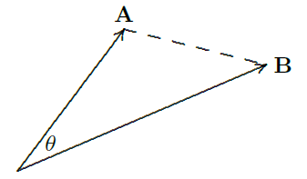
Since the angle \(\theta\) lies in a triangle, we can compute it using a bit of trigonometry, namely, the law of cosines. The lengths of the sides of the triangle in figure 12.3.1 are \(|{\bf A}|\), \(|{\bf B}|\), and \(|{\bf A}-{\bf B}|\). Let

\[ {\bf A}=\langle a_1,a_2,a_3\rangle\]

and

\[ {\bf B}=\langle b_1,b_2,b_3\rangle\]

then

\[\eqalign{ |{\bf A}-{\bf B}|^2&=|{\bf A}|^2+|{\bf B}|^2-2|{\bf A}||{\bf B}|\cos\theta\cr 2|{\bf A}||{\bf B}|\cos\theta&=|{\bf A}|^2+|{\bf B}|^2-|{\bf A}-{\bf B}|^2\cr &=a_1^2+a_2^2+a_3^2+b_1^2+b_2^2+b_3^2-(a_1-b_1)^2-(a_2-b_2)^2-(a_3-b_3)^2\cr &=a_1^2+a_2^2+a_3^2+b_1^2+b_2^2+b_3^2\cr &\qquad-(a_1^2-2a_1b_1+b_1^2) -(a_2^2-2a_2b_2+b_2^2)-(a_3^2-2a_3b_3+b_3^2)\cr &=2a_1b_1+2a_2b_2+2a_3b_3\cr |{\bf A}||{\bf B}|\cos\theta&=a_1b_1+a_2b_2+a_3b_3\cr \cos\theta&=(a_1b_1+a_2b_2+a_3b_3)/(|{\bf A}||{\bf B}|)\cr }\]

So a bit of simple arithmetic with the coordinates of \(\bf A\) and \(\bf B\) allows us to compute the cosine of the angle between them. If necessary we can use the arccosine to get \(\theta\), but in many problems \(\cos\theta\) turns out to be all we really need.

The numerator of the fraction that gives us \(\cos\theta\) turns up a lot, so we give it a name and more compact notation: we call it the dot product, and write it as

\[{\bf A}\cdot{\bf B} = a_1b_1+a_2b_2+a_3b_3.\]

This is the same symbol we use for ordinary multiplication, but there should never be any confusion; you can tell from context whether we are "multiplying'' vectors or numbers. (We might also use the dot for scalar multiplication: \(a\cdot{\bf V}=a{\bf V}\); again, it is clear what is meant from context.)

Example 12.3.1

Find the angle between the vectors \({\bf A}=\langle 1,2,1\rangle\) and \({\bf B}=\langle 3,1,-5\rangle\). We know that

\[\cos\theta={\bf A}\cdot{\bf B}/(|{\bf A}||{\bf B}|)= (1\cdot3 + 2\cdot1 + 1\cdot(-5))/(|{\bf A}||{\bf B}|)=0,\]

so \(\theta=\pi/2\), that is, the vectors are perpendicular.

Example 12.3.2

Find the angle between the vectors \({\bf A}=\langle 3,3,0\rangle\) and \({\bf B}=\langle 1,0,0\rangle\). We compute

\[\eqalign{ \cos\theta &= (3\cdot1 + 3\cdot0 + 0\cdot0)/(\sqrt{9+9+0}\sqrt{1+0+0})\cr &= 3/\sqrt{18} = 1/\sqrt2\cr}\]

so \(\theta=\pi/4\).

Example 12.3.3

Some special cases are worth looking at: Find the angles between \({\bf A}\) and \({\bf A}\); \({\bf A}\) and \({\bf -A}\); \({\bf A}\) and \({\bf 0}=\langle 0,0,0\rangle\).

\[ \cos\theta= {\bf A}\cdot{\bf A}/(|{\bf A}||{\bf A}|)=(a_1^2+a_2^2+a_3^2)/ (\sqrt{a_1^2+a_2^2+a_3^2}\sqrt{a_1^2+a_2^2+a_3^2})=1,\]

so the angle between \({\bf A}\) and itself is zero, which of course is correct.

\[ \cos\theta={\bf A}\cdot{\bf -A}/(|{\bf A}||{\bf -A}|)=(-a_1^2-a_2^2-a_3^2)/ (\sqrt{a_1^2+a_2^2+a_3^2}\sqrt{a_1^2+a_2^2+a_3^2})=-1,\]

so the angle is \(\pi\), that is, the vectors point in opposite directions, as of course we already knew.

\[ \cos\theta= {\bf A}\cdot{\bf 0}/(|{\bf A}||{\bf 0}|)=(0+0+0)/ (\sqrt{a_1^2+a_2^2+a_3^2}\sqrt{0^2+0^2+0^2}),\]

which is undefined. On the other hand, note that since \({\bf A}\cdot{\bf 0}=0\) it looks at first as if \(\cos\theta\) will be zero, which as we have seen means that vectors are perpendicular; only when we notice that the denominator is also zero do we run into trouble. One way to "fix'' this is to adopt the convention that the zero vector \({\bf 0}\) is perpendicular to all vectors; then we can say in general that if \({\bf A}\cdot{\bf B}=0\), \(\bf A\) and \(\bf B\) are perpendicular.

Generalizing the examples, note the following useful facts:

1. If \(\bf A\) is parallel or anti-parallel to \(\bf B\) then \({\bf A}\cdot{\bf B}/(|{\bf A}||{\bf B}|)=\pm1\), and conversely, if \({\bf A}\cdot{\bf B}/(|{\bf A}||{\bf B}|)=1\), \(\bf A\) and \(\bf B\) are parallel, while if \({\bf A}\cdot{\bf B}/(|{\bf A}||{\bf B}|)=-1\), \(\bf A\) and \(\bf B\) are anti-parallel. (Vectors are parallel if they point in the same direction, anti-parallel if they point in opposite directions.)
2. If \(\bf A\) is perpendicular to \(\bf B\) then \({\bf A}\cdot{\bf B}/(|{\bf A}||{\bf B}|)=0\), and conversely if \({\bf A}\cdot{\bf B}/(|{\bf A}||{\bf B}|)=0\) then \(\bf A\) and \(\bf B\) are perpendicular.

Given two vectors, it is often useful to find the projection of one vector onto the other, because this turns out to have important meaning in many circumstances. More precisely, given \({\bf A}\) and \({\bf B}\), we seek a vector parallel to \(\bf B\) but with length determined by \(\bf A\) in a natural way, as shown in figure 12.3.2. \(\bf V\) is chosen so that the triangle formed by \(\bf A\), \(\bf V\), and \({\bf A}-{\bf V}\) is a right triangle.

Figure 12.3.2. \(\bf V\) is the projection of \(\bf A\) onto \(\bf B\).

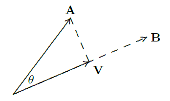
Using a little trigonometry, we see that

\[ |{\bf V}|=|{\bf A}|\cos\theta= |{\bf A}|{{\bf A}\cdot{\bf B}\over|{\bf A}||{\bf B}|}= {{\bf A}\cdot{\bf B}\over|{\bf B}|}; \]

this is sometimes called the scalar projection of \(\bf A\) onto \(\bf B\). To get \(\bf V\) itself, we multiply this length by a vector of length one parallel to \(\bf B\):

\[{\bf V}= {{\bf A}\cdot{\bf B}\over|{\bf B}|}{{\bf B}\over|{\bf B}|}= {{\bf A}\cdot{\bf B}\over|{\bf B}|^2}{\bf B}. \]

Be sure that you understand why \({\bf B}/|{\bf B}|\) is a vector of length one (also called a unit vector) parallel to \(\bf B\).

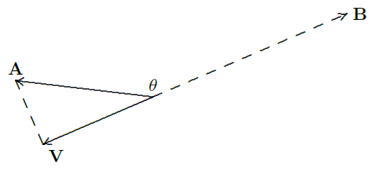
The discussion so far implicitly assumed that \(0\le\theta\le\pi/2\). If \(\pi/2 < \theta\le\pi\), the picture is like figure 12.3.3. In this case \({\bf A}\cdot {\bf B}\) is negative, so the vector

\[{{\bf A}\cdot{\bf B}\over|{\bf B}|^2}{\bf B}\]

is anti-parallel to \(\bf B\), and its length is

\[\left|{{\bf A}\cdot{\bf B}\over|{\bf B}|}\right|.\]

So in general, the scalar projection of \(\bf A\) onto \(\bf B\) may be positive or negative. If it is negative, it means that the projection vector is anti-parallel to \(\bf B\) and that the length of the projection vector is the absolute value of the scalar projection. Of course, you can also compute the length of the projection vector as usual, by applying the distance formula to the vector.

Figure 12.3.3. \(\bf V\) is the projection of \(\bf A\) onto \(\bf B\).

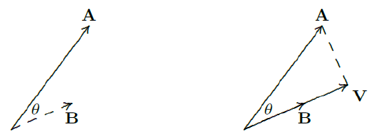
Note that the phrase "projection onto \(\bf B\)'' is a bit misleading if taken literally; all that \(\bf B\) provides is a direction; the length of \(\bf B\) has no impact on the final vector. In figure 12.3.4, for example, \(\bf B\) is shorter than the projection vector, but this is perfectly acceptable.

Figure 12.3.4. \(\bf V\) is the projection of \(\bf A\) onto \(\bf B\).

Example 12.3.4

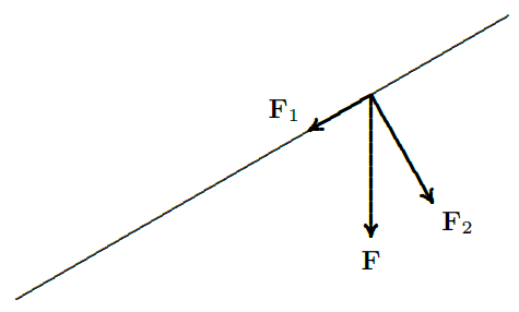
Physical force is a vector quantity. It is often necessary to compute the "component'' of a force acting in a different direction than the force is being applied. For example, suppose a ten pound weight is resting on an inclined plane---a pitched roof, for example. Gravity exerts a force of ten pounds on the object, directed straight down. It is useful to think of the component of this force directed down and parallel to the roof, and the component down and directly into the roof. These forces are the projections of the force vector onto vectors parallel and perpendicular to the roof. Suppose the roof is tilted at a \( 30^\circ\) angle, as in figure 12.3.5.

A vector parallel to the roof is \( \langle-\sqrt3,-1\rangle\), and a vector perpendicular to the roof is \( \langle 1,-\sqrt3\rangle\). The force vector is \({\bf F}=\langle 0,-10\rangle\). The component of the force directed down the roof is then

\[\eqalign{ {\bf F}_1&={{\bf F}\cdot \langle-\sqrt3,-1\rangle\over|\langle-\sqrt3,-1\rangle|^2} \langle-\sqrt3,-1\rangle ={10\over 2}{\langle-\sqrt3,-1\rangle\over2}= \langle -5\sqrt3/2,-5/2\rangle\cr }\]

with length 5. The component of the force directed into the roof is

\[\eqalign{ {\bf F}_2&={{\bf F}\cdot \langle1,-\sqrt3\rangle\over|\langle1,-\sqrt3\rangle|^2} \langle1,-\sqrt3\rangle ={10\sqrt3\over 2}{\langle1,-\sqrt3\rangle\over2}= \langle 5\sqrt3/2,-15/2\rangle\cr }\]

with length \( 5\sqrt3\). Thus, a force of 5 pounds is pulling the object down the roof, while a force of \( 5\sqrt3\) pounds is pulling the object into the roof.

Figure 12.3.5. Components of a force.

The dot product has some familiar-looking properties that will be useful later, so we list them here. These may be proved by writing the vectors in coordinate form and then performing the indicated calculations; subsequently it can be easier to use the properties instead of calculating with coordinates.

Theroem 12.3.5

If \({\bf u}\), \({\bf v}\), and \({\bf w}\) are vectors and \(a\) is a real number, then

1. \( {\bf u}\cdot{\bf u} = |{\bf u}|^2\)
2. \({\bf u}\cdot{\bf v} = {\bf v}\cdot{\bf u}\)
3. \({\bf u}\cdot({\bf v}+{\bf w}) = {\bf u}\cdot{\bf v}+{\bf u}\cdot{\bf w}\)
4. \((a{\bf u})\cdot{\bf v}=a({\bf u}\cdot{\bf v}) ={\bf u}\cdot(a{\bf v})\)

Contributors

David Guichard (Whitman College)

• Integrated by Justin Marshall.