1.4: One Sided Limits

Last updated
Save as PDF

Page ID: 4153

$ \newcommand{\vecs}[1]{\overset { \scriptstyle \rightharpoonup} {\mathbf{#1}} } $

$ \newcommand{\vecd}[1]{\overset{-\!-\!\rightharpoonup}{\vphantom{a}\smash {#1}}} $

$ \newcommand{\id}{\mathrm{id}}$ $ \newcommand{\Span}{\mathrm{span}}$

( \newcommand{\kernel}{\mathrm{null}\,}\) $ \newcommand{\range}{\mathrm{range}\,}$

$ \newcommand{\RealPart}{\mathrm{Re}}$ $ \newcommand{\ImaginaryPart}{\mathrm{Im}}$

$ \newcommand{\Argument}{\mathrm{Arg}}$ $ \newcommand{\norm}[1]{\| #1 \|}$

$ \newcommand{\inner}[2]{\langle #1, #2 \rangle}$

$ \newcommand{\Span}{\mathrm{span}}$

$ \newcommand{\id}{\mathrm{id}}$

$ \newcommand{\Span}{\mathrm{span}}$

$ \newcommand{\kernel}{\mathrm{null}\,}$

$ \newcommand{\range}{\mathrm{range}\,}$

$ \newcommand{\RealPart}{\mathrm{Re}}$

$ \newcommand{\ImaginaryPart}{\mathrm{Im}}$

$ \newcommand{\Argument}{\mathrm{Arg}}$

$ \newcommand{\norm}[1]{\| #1 \|}$

$ \newcommand{\inner}[2]{\langle #1, #2 \rangle}$

$ \newcommand{\Span}{\mathrm{span}}$ $ \newcommand{\AA}{\unicode[.8,0]{x212B}}$

$ \newcommand{\vectorA}[1]{\vec{#1}} % arrow$

$ \newcommand{\vectorAt}[1]{\vec{\text{#1}}} % arrow$

$ \newcommand{\vectorB}[1]{\overset { \scriptstyle \rightharpoonup} {\mathbf{#1}} } $

$ \newcommand{\vectorC}[1]{\textbf{#1}} $

$ \newcommand{\vectorD}[1]{\overrightarrow{#1}} $

$ \newcommand{\vectorDt}[1]{\overrightarrow{\text{#1}}} $

$ \newcommand{\vectE}[1]{\overset{-\!-\!\rightharpoonup}{\vphantom{a}\smash{\mathbf {#1}}}} $

$ \newcommand{\vecs}[1]{\overset { \scriptstyle \rightharpoonup} {\mathbf{#1}} } $

$ \newcommand{\vecd}[1]{\overset{-\!-\!\rightharpoonup}{\vphantom{a}\smash {#1}}} $

$\newcommand{\avec}{\mathbf a}$ $\newcommand{\bvec}{\mathbf b}$ $\newcommand{\cvec}{\mathbf c}$ $\newcommand{\dvec}{\mathbf d}$ $\newcommand{\dtil}{\widetilde{\mathbf d}}$ $\newcommand{\evec}{\mathbf e}$ $\newcommand{\fvec}{\mathbf f}$ $\newcommand{\nvec}{\mathbf n}$ $\newcommand{\pvec}{\mathbf p}$ $\newcommand{\qvec}{\mathbf q}$ $\newcommand{\svec}{\mathbf s}$ $\newcommand{\tvec}{\mathbf t}$ $\newcommand{\uvec}{\mathbf u}$ $\newcommand{\vvec}{\mathbf v}$ $\newcommand{\wvec}{\mathbf w}$ $\newcommand{\xvec}{\mathbf x}$ $\newcommand{\yvec}{\mathbf y}$ $\newcommand{\zvec}{\mathbf z}$ $\newcommand{\rvec}{\mathbf r}$ $\newcommand{\mvec}{\mathbf m}$ $\newcommand{\zerovec}{\mathbf 0}$ $\newcommand{\onevec}{\mathbf 1}$ $\newcommand{\real}{\mathbb R}$ $\newcommand{\twovec}[2]{\left[\begin{array}{r}#1 \\ #2 \end{array}\right]}$ $\newcommand{\ctwovec}[2]{\left[\begin{array}{c}#1 \\ #2 \end{array}\right]}$ $\newcommand{\threevec}[3]{\left[\begin{array}{r}#1 \\ #2 \\ #3 \end{array}\right]}$ $\newcommand{\cthreevec}[3]{\left[\begin{array}{c}#1 \\ #2 \\ #3 \end{array}\right]}$ $\newcommand{\fourvec}[4]{\left[\begin{array}{r}#1 \\ #2 \\ #3 \\ #4 \end{array}\right]}$ $\newcommand{\cfourvec}[4]{\left[\begin{array}{c}#1 \\ #2 \\ #3 \\ #4 \end{array}\right]}$ $\newcommand{\fivevec}[5]{\left[\begin{array}{r}#1 \\ #2 \\ #3 \\ #4 \\ #5 \\ \end{array}\right]}$ $\newcommand{\cfivevec}[5]{\left[\begin{array}{c}#1 \\ #2 \\ #3 \\ #4 \\ #5 \\ \end{array}\right]}$ $\newcommand{\mattwo}[4]{\left[\begin{array}{rr}#1 \amp #2 \\ #3 \amp #4 \\ \end{array}\right]}$ $\newcommand{\laspan}[1]{\text{Span}\{#1\}}$ $\newcommand{\bcal}{\cal B}$ $\newcommand{\ccal}{\cal C}$ $\newcommand{\scal}{\cal S}$ $\newcommand{\wcal}{\cal W}$ $\newcommand{\ecal}{\cal E}$ $\newcommand{\coords}[2]{\left\{#1\right\}_{#2}}$ $\newcommand{\gray}[1]{\color{gray}{#1}}$ $\newcommand{\lgray}[1]{\color{lightgray}{#1}}$ $\newcommand{\rank}{\operatorname{rank}}$ $\newcommand{\row}{\text{Row}}$ $\newcommand{\col}{\text{Col}}$ $\renewcommand{\row}{\text{Row}}$ $\newcommand{\nul}{\text{Nul}}$ $\newcommand{\var}{\text{Var}}$ $\newcommand{\corr}{\text{corr}}$ $\newcommand{\len}[1]{\left|#1\right|}$ $\newcommand{\bbar}{\overline{\bvec}}$ $\newcommand{\bhat}{\widehat{\bvec}}$ $\newcommand{\bperp}{\bvec^\perp}$ $\newcommand{\xhat}{\widehat{\xvec}}$ $\newcommand{\vhat}{\widehat{\vvec}}$ $\newcommand{\uhat}{\widehat{\uvec}}$ $\newcommand{\what}{\widehat{\wvec}}$ $\newcommand{\Sighat}{\widehat{\Sigma}}$ $\newcommand{\lt}{<}$ $\newcommand{\gt}{>}$ $\newcommand{\amp}{&}$ $\definecolor{fillinmathshade}{gray}{0.9}$

We introduced the concept of a limit gently, approximating their values graphically and numerically. Next came the rigorous definition of the limit, along with an admittedly tedious method for evaluating them. The previous section gave us tools (which we call theorems) that allow us to compute limits with greater ease. Chief among the results were the facts that polynomials and rational, trigonometric, exponential and logarithmic functions (and their sums, products, etc.) all behave "nicely.'' In this section we rigorously define what we mean by "nicely.''

In Section 1.1 we explored the three ways in which limits of functions failed to exist:

The function approached different values from the left and right,
The function grows without bound, and
The function oscillates.

In this section we explore in depth the concepts behind #1 by introducing the one-sided limit. We begin with formal definitions that are very similar to the definition of the limit given in Section 1.2, but the notation is slightly different and "$x\neq c$'' is replaced with either "$x<c$'' or "$x>c$.''

Definition 2: One Sided Limits

Left-Hand Limit

Let $I$ be an open interval containing $c$, and let $f$ be a function defined on $I$, except possibly at $c$. The limit of $f(x)$, as $x$ approaches $c$ from the left, is $L$, or, the left--hand limit of $f$ at $c$ is $L$, denoted by

\[ \lim\limits_{x\rightarrow c^-} f(x) = L,\]

means that given any $\epsilon > 0$, there exists $\delta > 0$ such that for all $x< c$, if $|x - c| < \delta$, then $|f(x) - L| < \epsilon$.

Right-Hand Limit

Let $I$ be an open interval containing $c$, and let $f$ be a function defined on $I$, except possibly at $c$. The limit of $f(x)$, as $x$ approaches $c$ from the right, is $L$, or, the right--hand limit of $f$ at $c$ is $L$, denoted by

\[ \lim\limits_{x\rightarrow c^+} f(x) = L,\]

means that given any $\epsilon > 0$, there exists $\delta > 0$ such that for all $x> c$, if $|x - c| < \delta$, then $|f(x) - L| < \epsilon$.

Practically speaking, when evaluating a left-hand limit, we consider only values of $x$ "to the left of $c$,'' i.e., where $x<c$. The admittedly imperfect notation $x\to c^-$ is used to imply that we look at values of $x$ to the left of $c$. The notation has nothing to do with positive or negative values of either $x$ or $c$. A similar statement holds for evaluating right-hand limits; there we consider only values of $x$ to the right of $c$, i.e., $x>c$. We can use the theorems from previous sections to help us evaluate these limits; we just restrict our view to one side of $c$.

We practice evaluating left and right-hand limits through a series of examples.

Example 17: Evaluating one sided limits

Let $ f(x) = \left\{\begin{array}{cc} x & 0\leq x\leq 1 \\ 3-x & 1<x<2\end{array},\right.$ as shown in Figure 1.21. Find each of the following:

$\lim\limits_{x\to 1^-} f(x)$
$\lim\limits_{x\to 1^+} f(x)$
$\lim\limits_{x\to 1} f(x)$
$f(1)$
$\lim\limits_{x\to 0^+} f(x) $
$f(0)$
$\lim\limits_{x\to 2^-} f(x)$
$f(2)$

$alt$
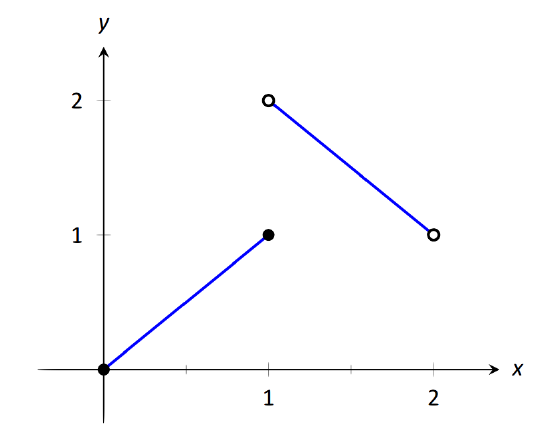
$\text{FIGURE 1.21}$: A graph of $f$ in Example 17.

Solution

For these problems, the visual aid of the graph is likely more effective in evaluating the limits than using $f$ itself. Therefore we will refer often to the graph.

As $x$ goes to 1 from the left, we see that $f(x)$ is approaching the value of 1. Therefore $ \lim\limits_{x\to 1^-} f(x) =1.$
As $x$ goes to 1 from the right, we see that $f(x)$ is approaching the value of 2. Recall that it does not matter that there is an "open circle'' there; we are evaluating a limit, not the value of the function. Therefore $ \lim\limits_{x\to 1^+} f(x)=2$.
The limit of $f$ as $x$ approaches 1 does not exist, as discussed in the first section. The function does not approach one particular value, but two different values from the left and the right.
Using the definition and by looking at the graph we see that $f(1) = 1$.
As $x$ goes to 0 from the right, we see that $f(x)$ is also approaching 0. Therefore $ \lim\limits_{x\to 0^+} f(x)=0$. Note we cannot consider a left-hand limit at 0 as $f$ is not defined for values of $x<0$.
Using the definition and the graph, $f(0) = 0$.
As $x$ goes to 2 from the left, we see that $f(x)$ is approaching the value of 1. Therefore $ \lim\limits_{x\to 2^-} f(x)=1.$
The graph and the definition of the function show that $f(2)$ is not defined.

Note how the left and right-hand limits were different at $x=1$. This, of course, causes the limit to not exist. The following theorem states what is fairly intuitive: the limit exists precisely when the left and right-hand limits are equal.

Theorem 7: Limits and One Sided Limits

Let $f$ be a function defined on an open interval $I$ containing $c$. Then \[\lim\limits_{x\to c}f(x) = L\]if, and only if, \[\lim\limits_{x\to c^-}f(x) = L \quad \text{and} \quad \lim\limits_{x\to c^+}f(x) = L.\]

The phrase "if, and only if'' means the two statements are equivalent: they are either both true or both false. If the limit equals $L$, then the left and right hand limits both equal $L$. If the limit is not equal to $L$, then at least one of the left and right-hand limits is not equal to $L$ (it may not even exist).

One thing to consider in Examples 17 - 20 is that the value of the function may/may not be equal to the value(s) of its left/right-hand limits, even when these limits agree.

Example 18: Evaluating limits of a piecewise-defined function

Let $f(x) = \left\{\begin{array}{cc} 2-x & 0<x<1 \\ (x-2)^2 & 1<x<2 \end{array},\right.$ as shown in Figure 1.22. Evaluate the following.

$ \lim\limits_{x\to 1^-} f(x)$
$ \lim\limits_{x\to 1^+} f(x)$
$ \lim\limits_{x\to 1} f(x)$
$ f(1)$
$ \lim\limits_{x\to 0^+} f(x)$
$f(0)$
$ \lim\limits_{x\to 2^-} f(x)$
$f(2)$

$alt$
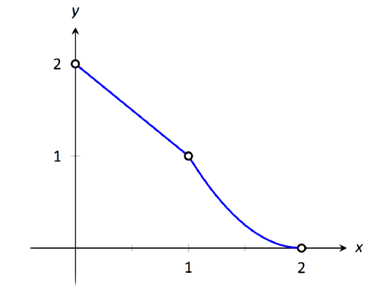
$\text{FIGURE 1.22}$: A graph of $f$ from Example 18.

Solution

Again we will evaluate each using both the definition of $f$ and its graph.

As $x$ approaches 1 from the left, we see that $f(x)$ approaches 1. Therefore $ \lim\limits_{x\to 1^-} f(x)=1.$
As $x$ approaches 1 from the right, we see that again $f(x)$ approaches 1. Therefore $ \lim\limits_{x\to 1+} f(x)=1$.
The limit of $f$ as $x$ approaches 1 exists and is 1, as $f$ approaches 1 from both the right and left. Therefore $ \lim\limits_{x\to 1} f(x)=1$.
$f(1)$ is not defined. Note that 1 is not in the domain of $f$ as defined by the problem, which is indicated on the graph by an open circle when $x=1$.
As $x$ goes to 0 from the right, $f(x)$ approaches 2. So $ \lim\limits_{x\to 0^+} f(x)=2$.
$f(0)$ is not defined as $0$ is not in the domain of $f$.
As $x$ goes to 2 from the left, $f(x)$ approaches 0. So $ \lim\limits_{x\to 2^-} f(x)=0$.
$f(2)$ is not defined as 2 is not in the domain of $f$.

Example 19: Evaluating limits of a piecewise-defined function

Let $f(x) = \left\{\begin{array}{cc} (x-1)^2 & 0\leq x\leq 2, x\neq 1\\ 1 & x=1\end{array},\right.$ as shown in Figure 1.23. Evaluate the following.

$ \lim\limits_{x\to 1^-} f(x)$
$ \lim\limits_{x\to 1^+} f(x)$
$ \lim\limits_{x\to 1} f(x)$
$f(1)$

$alt$
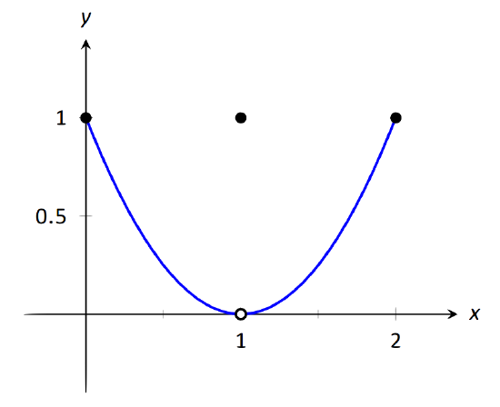
$\text{FIGURE 1.23}$: Graphing $f$ in Example 19.

It is clear by looking at the graph that both the left and right-hand limits of $f$, as $x$ approaches 1, is 0. Thus it is also clear that the limit is 0; i.e., $ \lim\limits_{x\to 1} f(x) = 0$. It is also clearly stated that $f(1) = 1$.

Example 20: Evaluating limits of a piecewise-defined function

Let $f(x) = \left\{\begin{array}{cc} x^2 & 0\leq x\leq 1 \\ 2-x & 1<x\leq 2\end{array},\right.$ as shown in Figure 1.24. Evaluate the following.

$ \lim\limits_{x\to 1^-} f(x)$
$ \lim\limits_{x\to 1^+} f(x)$
$ \lim\limits_{x\to 1} f(x)$
$f(1)$

$alt$
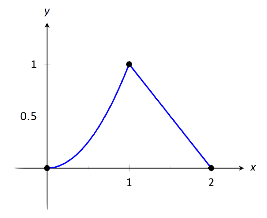
$\text{FIGURE 1.24}$: Graphing $f$ in Example 20.

Solution

It is clear from the definition of the function and its graph that all of the following are equal:

\[\lim\limits_{x\to 1^-} f(x) = \lim\limits_{x\to 1^+} f(x) =\lim\limits_{x\to 1} f(x) =f(1) = 1.\]

In Examples 17 - 20 we were asked to find both $ \lim\limits_{x\to 1}f(x)$ and $f(1)$. Consider the following table:

\[\begin{array}{ccc} & \lim\limits_{x\to 1}f(x) & f(1) \\ \hline \text{Example 17} & \text{does not exist} & 1 \\ \text{Example 18} & 1 & \text{not defined} \\ \text{Example 19} & 0 & 1 \\ \text{Example 20} & 1 & 1 \\ \end{array}\]

Only in Example 20 do both the function and the limit exist and agree. This seems "nice;'' in fact, it seems "normal.'' This is in fact an important situation which we explore in the next section, entitled "Continuity.'' In short, a continuous function is one in which when a function approaches a value as $x\rightarrow c$ (i.e., when $ \lim\limits_{x\to c} f(x) = L$), it actually attains that value at $c$. Such functions behave nicely as they are very predictable.

Contributors and Attributions

Gregory Hartman (Virginia Military Institute). Contributions were made by Troy Siemers and Dimplekumar Chalishajar of VMI and Brian Heinold of Mount Saint Mary's University. This content is copyrighted by a Creative Commons Attribution - Noncommercial (BY-NC) License. http://www.apexcalculus.com/

Search

Text Color

Text Size

Margin Size

Font Type