1.5: Continuity

As we have studied limits, we have gained the intuition that limits measure ``where a function is heading.'' That is, if

\[ \lim\limits_{x\to 1} f(x) = 3\]

then as \(x\) is close to 1, \(f(x)\) is close to 3. We have seen, though, that this is not necessarily a good indicator of what \(f(1)\) actually is. This can be problematic; functions can tend to one value but attain another. This section focuses on functions that do not exhibit such behavior.

Definition 3 Continuous Function

Let \(f\) be a function defined on an open interval \(I\) containing \(c\).

1. \(f\) is continuous at \(c\) if \( \lim\limits_{x\to c}f(x) = f(c)\).
2. \(f\) is continuous on \(I\) if \(f\) is continuous at \(c\) for all values of \(c\) in \(I\). If \(f\) is continuous on \((-\infty,\infty)\), we say \(f\) is continuous everywhere.

A useful way to establish whether or not a function \(f\) is continuous at \(c\) is to verify the following three things:

1. \( \lim\limits_{x\to c} f(x)\) exists,
2. \(f(c)\) is defined, and
3. \( \lim\limits_{x\to c} f(x) = f(c)\).

Example 21: Finding intervals of continuity

Let \(f\) be defined as shown in Figure 1.25. Give the interval(s) on which \(f\) is continuous.

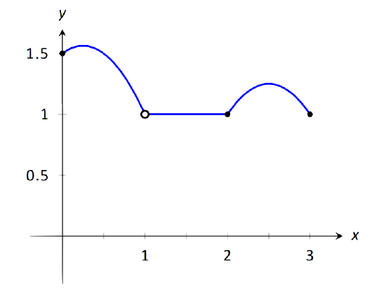
\(\text{FIGURE 1.25}\): A graph of \(f\) in Example 21.

Solution

We proceed by examining the three criteria for continuity.

1. The limits \( \lim\limits_{x\to c} f(x)\) exists for all \(c\) between 0 and 3.
2. \(f(c)\) is defined for all \(c\) between 0 and 3, except for \(c=1\). We know immediately that \(f\) cannot be continuous at \(x=1\).
3. The limit \( \lim\limits_{x\to c} f(x) = f(c)\) for all \(c\) between 0 and 3, except, of course, for \(c=1\).

We conclude that \(f\) is continuous at every point of \((0,3)\) except at \(x=1\). Therefore \(f\) is continuous on \((0,1)\cup(1,3)\).

Example 22: Finding intervals of continuity

The floor function, \(f(x) = \lfloor x \rfloor\), returns the largest integer smaller than the input \(x\). (For example, \(f(\pi) = \lfloor \pi \rfloor = 3\).) The graph of \(f\) in Figure 1.26 demonstrates why this is often called a "step function.''

Give the intervals on which \(f\) is continuous.

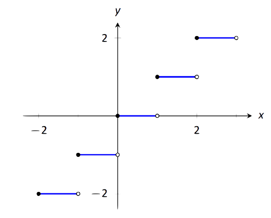
\(\text{FIGURE 1.26}\): A graph of the step function in Example 22.

Solution

We examine the three criteria for continuity.

1. The limits \(\lim\limits_{x\to c} f(x)\) do not exist at the jumps from one "step'' to the next, which occur at all integer values of \(c\). Therefore the limits exist for all \(c\) except when \(c\) is an integer.
2. The function is defined for all values of \(c\).
3. The limit \( \lim\limits_{x\to c} f(x) = f(c)\) for all values of \(c\) where the limit exist, since each step consists of just a line.

We conclude that \(f\) is continuous everywhere except at integer values of \(c\). So the intervals on which \(f\) is continuous are \[\ldots, (-2,-1), (-1,0), (0,1), (1,2), \ldots.\]

Our definition of continuity on an interval specifies the interval is an open interval. We can extend the definition of continuity to closed intervals by considering the appropriate one-sided limits at the endpoints.

Definition 4: Continuity on Closed Intervals

Let \(f\) be defined on the closed interval \([a,b]\) for some real numbers \(a,b\). \(f\) is continuous on \([a,b]\) if:

1. \(f\) is continuous on \((a,b)\),
2. \( \lim\limits_{x\to a^+} f(x) = f(a)\) and
3. \( \lim\limits_{x\to b^-} f(x) = f(b)\).

We can make the appropriate adjustments to talk about continuity on half--open intervals such as \([a,b)\) or \((a,b]\) if necessary.

Example 23: Determining intervals on which a function is continuous

For each of the following functions, give the domain of the function and the interval(s) on which it is continuous.

1. \(f(x) = 1/x\)
2. \(f(x) = \sin x\)
3. \(f(x) = \sqrt{x}\)
4. \(f(x) = \sqrt{1-x^2}\)
5. \(f(x) = |x|\)

Solution

We examine each in turn.

1. The domain of \(f(x) = 1/x\) is \((-\infty,0) \cup (0,\infty)\). As it is a rational function, we apply Theorem 2 to recognize that \(f\) is continuous on all of its domain.
2. The domain of \(f(x) = \sin x\) is all real numbers, or \((-\infty,\infty)\). Applying Theorem 3 shows that \(\sin x\) is continuous everywhere.
3. The domain of \(f(x) = \sqrt{x}\) is \([0,\infty)\). Applying Theorem 3 shows that \(f(x) = \sqrt{x}\) is continuous on its domain of \([0,\infty)\).
4. The domain of \(f(x) = \sqrt{1-x^2}\) is \([-1,1]\). Applying Theorems 1 and 3 shows that \(f\) is continuous on all of its domain, \([-1,1]\).
5. The domain of \(f(x) = |x|\) is \((-\infty,\infty)\). We can define the absolute value function as \( f(x) = \left\{\begin{array}{cc} -x & x<0 \\ x & x\geq 0\end{array}\right. \). Each "piece'' of this piecewise defined function is continuous on all of its domain, giving that \(f\) is continuous on \((-\infty,0)\) and \([0,\infty)\). We cannot assume this implies that \(f\) is continuous on \((-\infty,\infty)\); we need to check that \( \lim\limits_{x\to 0}f(x) = f(0)\), as \(x=0\) is the point where \(f\) transitions from one ``piece'' of its definition to the other. It is easy to verify that this is indeed true, hence we conclude that \(f(x) = |x|\) is continuous everywhere.

Continuity is inherently tied to the properties of limits. Because of this, the properties of limits found in Theorems 1 and 2 apply to continuity as well. Further, now knowing the definition of continuity we can re--read Theorem 3 as giving a list of functions that are continuous on their domains. The following theorem states how continuous functions can be combined to form other continuous functions, followed by a theorem which formally lists functions that we know are continuous on their domains.

Theorem 8: Properties of Continuous Functions

Let \(f\) and \(g\) be continuous functions on an interval \(I\), let \(c\) be a real number and let \(n\) be a positive integer. The following functions are continuous on \(I\).

1. Sums/Differences : \(f\pm g\)
2. Constant Multiples : \(c\cdot f\)
3. Products : \(f\cdot g\)
4. Quotients : \(f/g\) (as long as \(g\neq 0\) on \(I\))
5. Powers : \(f\,^n\)
6. Roots : \(\sqrt[n]{f}\) (if \(n\) is even then \(f\geq 0\) on \(I\); if \(n\) is odd, then true for all values of \(f\) on \(I\).)
7. Compositions : Adjust the definitions of \(f\) and \(g\) to: Let \(f\) be continuous on \(I\), where the range of \(f\) on \(I\) is \(J\), and let \(g\) be continuous on \(J\). Then \(g\circ f\), i.e., \(g(f(x))\), is continuous on \(I\).

Theorem 9: Continuous Functions

The following functions are continuous on their domains.

\(\begin{align} &1.\, f(x) = \sin x \qquad \qquad \qquad &&2.\, f(x) = \cos x \\ &3.\,f(x) = \tan x &&4.\,f(x) = \cot x \\ &5.\,f(x) = \sec x &&6.\,f(x) = \csc x \\ &7.\,f(x) = \ln x &&8.\,f(x) = \sqrt[n]{x}, \\ &9.\,f(x) = a^x (a>0) &&\,\,\, \text{(where n is a positive integer)} \\ \end{align}\)

We apply these theorems in the following Example.

Example 24: Determining intervals on which a function is continuous

State the interval(s) on which each of the following functions is continuous.

\(\begin{align}&1.\,\,f(x) = \sqrt{x-1} + \sqrt{5-x} \qquad \qquad \qquad &&3.\,\,f(x) = \tan x \\ &2.\,\,f(x) = x\sin x &&4.\,\, f(x) = \sqrt{\ln x} \\ \end{align}\)

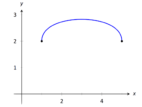
\(\text{FIGURE 1.27}\): A graph of \(f\) in Example 24(a).

Solution

We examine each in turn, applying Theorems 8 and 9 as appropriate.

1. The square--root terms are continuous on the intervals \([1,\infty)\) and \((-\infty,5]\), respectively. As \(f\) is continuous only where each term is continuous, \(f\) is continuous on \([1,5]\), the intersection of these two intervals. A graph of \(f\) is given in Figure 1.27.
   
2. The functions \(y=x\) and \(y=\sin x\) are each continuous everywhere, hence their product is, too.
3. Theorem 9 states that \(f(x) = \tan x\) is continuous "on its domain.'' Its domain includes all real numbers except odd multiples of \(\pi/2\). Thus \(f(x) = \tan x\) is continuous on \[\ldots \left(-\frac{3\pi}{2},-\frac{\pi}2\right),\ \left(-\frac{\pi}2,\frac{\pi}2\right),\ \left(\frac{\pi}2,\frac{3\pi}2\right),\ldots,\]or, equivalently, on \(D = \{x\in \mathbb{R}\ |\ x\neq n\cdot \frac{\pi}2,\, \text{n is an odd integer} \}.\)
4. The domain of \(y = \sqrt{x}\) is \([0,\infty)\). The range of \(y=\ln x\) is \((-\infty,\infty)\), but if we restrict its domain to \([1,\infty)\) its range is \([0,\infty)\). So restricting \(y = \ln x\) to the domain of \([1,\infty)\) restricts its output is \([0,\infty)\), on which \(y = \sqrt{x}\) is defined. Thus the domain of \(f(x) = \sqrt{\ln x}\) is \([1,\infty)\).

A common way of thinking of a continuous function is that "its graph can be sketched without lifting your pencil.'' That is, its graph forms a "continuous'' curve, without holes, breaks or jumps. While beyond the scope of this text, this pseudo--definition glosses over some of the finer points of continuity. Very strange functions are continuous that one would be hard pressed to actually sketch by hand.

This intuitive notion of continuity does help us understand another important concept as follows. Suppose \(f\) is defined on \([1,2]\) and \(f(1) = -10\) and \(f(2) = 5\). If \(f\) is continuous on \([1,2]\) (i.e., its graph can be sketched as a continuous curve from \((1,-10)\) to \((2,5)\)) then we know intuitively that somewhere on \([1,2]\) \(f\) must be equal to \(-9\), and \(-8\), and \(-7,\ -6,\ \ldots,\ 0,\ 1/2,\) etc. In short, \(f\) takes on all intermediate values between \(-10\) and \(5\). It may take on more values; \(f\) may actually equal 6 at some time, for instance, but we are guaranteed all values between \(-10\) and 5.

While this notion seems intuitive, it is not trivial to prove and its importance is profound. Therefore the concept is stated in the form of a theorem.

Theorem 10: Intermediate Value Theorem

Let \(f\) be a continuous function on \([a,b]\) and, without loss of generality, let \(f(a) < f(b)\). Then for every value \(y\), where \(f(a) < y < f(b)\), there is a value \(c\) in \([a,b]\) such that \(f(c) = y\).

One important application of the Intermediate Value Theorem is root finding. Given a function \(f\), we are often interested in finding values of \(x\) where \(f(x) = 0\). These roots may be very difficult to find exactly. Good approximations can be found through successive applications of this theorem. Suppose through direct computation we find that \(f(a) <0 \( and \(f(b)>0\), where \(a<b\). The Intermediate Value Theorem states that there is a \(c\) in \([a,b]\) such that \(f(c) = 0\). The theorem does not give us any clue as to where that value is in the interval \([a,b]\), just that it exists.

There is a technique that produces a good approximation of \(c\). Let \(d\) be the midpoint of the interval \([a,b]\) and consider \(f(d)\). There are three possibilities:

1. \(f(d) = 0\) -- we got lucky and stumbled on the actual value. We stop as we found a root.
2. \(f(d) <0\) Then we know there is a root of \(f\) on the interval \([d,b]\) -- we have halved the size of our interval, hence are closer to a good approximation of the root.
3. \(f(d) >0\) Then we know there is a root of \(f\) on the interval \([a,d]\) -- again,we have halved the size of our interval, hence are closer to a good approximation of the root.

Successively applying this technique is called the Bisection Method of root finding. We continue until the interval is sufficiently small. We demonstrate this in the following example.

Example 25: Using the Bisection Method

Approximate the root of \(f(x) = x-\cos x\), accurate to three places after the decimal.

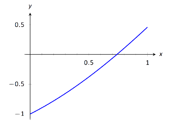
\(\text{FIGURE 1.28}\): Graphing a root of \(f(x) = x-\cos x\).

Solution

Consider the graph of \(f(x) = x-\cos x\), shown in Figure 1.28. It is clear that the graph crosses the \(x\)-axis somewhere near \(x=0.8\). To start the Bisection Method, pick an interval that contains \(0.8\). We choose \([0.7,0.9]\). Note that all we care about are signs of \(f(x)\), not their actual value, so this is all we display.

1. Iteration 1: \(f(0.7) < 0\), \(f(0.9) > 0\), and \(f(0.8) >0\). So replace \(0.9\) with \(0.8\) and repeat.
2. Iteration 2: \(f(0.7)<0\), \(f(0.8) > 0\), and at the midpoint, \(0.75\), we have \(f(0.75) >0 \). So replace \(0.8\) with \(0.75\) and repeat. Note that we don't need to continue to check the endpoints, just the midpoint. Thus we put the rest of the iterations in Table 1.29.

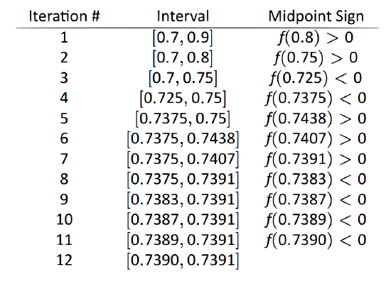
\(\text{FIGURE 1.29}\): Iterations of the Bisection Method of Root Finding

Notice that in the 12\(^\text{th}\) iteration we have the endpoints of the interval each starting with \(0.739\). Thus we have narrowed the zero down to an accuracy of the first three places after the decimal. Using a computer, we have

\[ f(0.7390) = -0.00014, \quad f(0.7391) = 0.000024.\]Either endpoint of the interval gives a good approximation of where \(f\) is 0. The Intermediate Value Theorem states that the actual zero is still within this interval. While we do not know its exact value, we know it starts with \(0.739\).

This type of exercise is rarely done by hand. Rather, it is simple to program a computer to run such an algorithm and stop when the endpoints differ by a preset small amount. One of the authors did write such a program and found the zero of \(f\), accurate to 10 places after the decimal, to be 0.7390851332. While it took a few minutes to write the program, it took less than a thousandth of a second for the program to run the necessary 35 iterations. In less than 8 hundredths of a second, the zero was calculated to 100 decimal places (with less than 200 iterations).

It is a simple matter to extend the Bisection Method to solve problems similar to "Find \(x\), where \(f(x) = 0\).'' For instance, we can find \(x\), where \(f(x) = 1\). It actually works very well to define a new function \(g\) where \(g(x) = f(x) - 1\). Then use the Bisection Method to solve \(g(x)=0\).

Similarly, given two functions \(f\) and \(g\), we can use the Bisection Method to solve \(f(x) = g(x)\). Once again, create a new function \(h\) where \(h(x) = f(x)-g(x)\) and solve \(h(x) = 0\).

In Section 4.1 another equation solving method will be introduced, called Newton's Method. In many cases, Newton's Method is much faster. It relies on more advanced mathematics, though, so we will wait before introducing it.

This section formally defined what it means to be a continuous function. "Most'' functions that we deal with are continuous, so often it feels odd to have to formally define this concept. Regardless, it is important, and forms the basis of the next chapter.

In the next section we examine one more aspect of limits: limits that involve infinity.

Contributors and Attributions

• Gregory Hartman (Virginia Military Institute). Contributions were made by Troy Siemers and Dimplekumar Chalishajar of VMI and Brian Heinold of Mount Saint Mary's University. This content is copyrighted by a Creative Commons Attribution - Noncommercial (BY-NC) License. http://www.apexcalculus.com/