4.2: Related Rates

When two quantities are related by an equation, knowing the value of one quantity can determine the value of the other. For instance, the circumference and radius of a circle are related by \(C=2\pi r\); knowing that \(C = 6\pi\) in determines the radius must be 3 in.

The topic of related rates takes this one step further: knowing the rate at which one quantity is changing can determine the rate at which the other changes.

Note: This section relies heavily on implicit differentiation, so referring back to Section 2.6 may help. We demonstrate the concepts of related rates through examples.

Example \(\PageIndex{1}\): Understanding related rates

The radius of a circle is growing at a rate of 5 in/hr. At what rate is the circumference growing?

Solution

The circumference and radius of a circle are related by \(C = 2\pi r\). We are given information about how the length of \(r\) changes with respect to time; that is, we are told \(\frac{dr}{dt} = 5\)in/hr. We want to know how the length of \(C\) changes with respect to time, i.e., we want to know \(\frac{dC}{dt}\).

Implicitly differentiate both sides of \(C = 2\pi r\) with respect to \(t\):

\[\begin{align*} C &= 2\pi r\\ \frac{d}{dt}\big(C\big) &= \frac{d}{dt}\big(2\pi r\big) \\ \frac{dC}{dt} &= 2\pi \frac{dr}{dt}.
\end{align*}\]

As we know \(\frac{dr}{dt} = 5\)in/hr, we know

$$\frac{dC}{dt} = 2\pi 5 = 10\pi \approx 31.4\text{in/hr.}\]

Consider another, similar example.

Example \(\PageIndex{2}\): Finding related rates

Water streams out of a faucet at a rate of \(2\)in\(^3\)/s onto a flat surface at a constant rate, forming a circular puddle that is \(1/8\)in deep.

1. At what rate is the area of the puddle growing?
2. At what rate is the radius of the circle growing?

Solution

1. We can answer this question two ways: using "common sense" or related rates. The common sense method states that the volume of the puddle is growing by \(2\)in\(^3\)/s, where

\[\text{volume of puddle}\, =\, \text{area of circle} \times \text{depth}.\]

Since the depth is constant at \(1/8\)in, the area must be growing by 16in\(^2\)/s.

This approach reveals the underlying related--rates principle. Let \(V\) and \(A\) represent the Volume and Area of the puddle. We know \(V= A\times \frac18\). Take the derivative of both sides with respect to \(t\), employing implicit differentiation.

\[\begin{align} V &= \frac18A\\ \frac{d}{dt}\big(V\big) &= \frac{d}{dt}\left(\frac18A\right)\\ \frac{dV}{dt} &= \frac18\frac{dA}{dt} \end{align}\]

As \(\frac{dV}{dt} = 2\), we know \(2 = \frac18\frac{dA}{dt}\), and hence \(\frac{dA}{dt} = 16\). Thus the area is growing by 16in\(^2\)/s.

2. To start, we need an equation that relates what we know to the radius. We just learned something about the surface area of the circular puddle, and we know \(A = \pi r^2\). We should be able to learn about the rate at which the radius is growing with this information.

Implicitly derive both sides of \(A=\pi r^2\) with respect to \(t\):

\[\begin{align} A &= \pi r^2 \\ \frac{d}{dt}\big(A\big) &= \frac{d}{dt}\big(\pi r^2\big)\\ \frac{dA}{dt} &= 2\pi r\frac{dr}{dt} \end{align}\]

Our work above told us that \(\frac{dA}{dt} = 16\text{in}^2\)/s. Solving for \(\frac{dr}{dt}\), we have

$$\frac{dr}{dt} = \frac{8}{\pi r}.\]

Note how our answer is not a number, but rather a function of \(r\). In other words, the rate at which the radius is growing depends on how big the circle already is. If the circle is very large, adding 2in\(^3\) of water will not make the circle much bigger at all. If the circle dime--sized, adding the same amount of water will make a radical change in the radius of the circle.

In some ways, our problem was (intentionally) ill--posed. We need to specify a current radius in order to know a rate of change. When the puddle has a radius of 10in, the radius is growing at a rate of

$$\frac{dr}{dt} = \frac{8}{10\pi} = \frac{4}{5\pi} \approx 0.25\text{in/s}.\]

Example \(\PageIndex{3}\): Studying related rates

Radar guns measure the rate of distance change between the gun and the object it is measuring. For instance, a reading of "55mph" means the object is moving away from the gun at a rate of 55 miles per hour, whereas a measurement of "\(-25\)mph" would mean that the object is approaching the gun at a rate of 25 miles per hour.

If the radar gun is moving (say, attached to a police car) then radar readouts are only immediately understandable if the gun and the object are moving along the same line. If a police officer is traveling 60mph and gets a readout of 15mph, he knows that the car ahead of him is moving away at a rate of 15 miles an hour, meaning the car is traveling 75mph. (This straight--line principle is one reason officers park on the side of the highway and try to shoot straight back down the road. It gives the most accurate reading.)

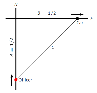
Suppose an officer is driving due north at 30 mph and sees a car moving due east, as shown in Figure \(\PageIndex{1}\). Using his radar gun, he measures a reading of 20mph. By using landmarks, he believes both he and the other car are about 1/2 mile from the intersection of their two roads.

Figure \(\PageIndex{1}\): A sketch of a police car (at bottom) attempting to measure the speed of a car (at right) in Example \(\PageIndex{3}\).

If the speed limit on the other road is 55mph, is the other driver speeding?

Solution

Using the diagram in Figure \(\PageIndex{1}\), let's label what we know about the situation. As both the police officer and other driver are 1/2 mile from the intersection, we have \(A = 1/2\), \(B = 1/2\), and through the Pythagorean Theorem, \(C = 1/\sqrt{2}\approx 0.707\).

We know the police officer is traveling at 30mph; that is, \(\frac{dA}{dt} = -30\). The reason this rate of change is negative is that \(A\) is getting smaller; the distance between the officer and the intersection is shrinking. The radar measurement is \(\frac{dC}{dt} = 20\). We want to find \(\frac{dB}{dt}\).

We need an equation that relates \(B\) to \(A\) and/or \(C\). The Pythagorean Theorem is a good choice: \(A^2+B^2 = C^2\). Differentiate both sides with respect to \(t\):

\[\begin{align} A^2 + B^2 &= C^2 \\ \frac{d}{dt}\left(A^2+B^2\right) &= \frac{d}{dt}\left(C^2\right) \\ 2A\frac{dA}{dt} + 2B\frac{dB}{dt} &= 2C\frac{dC}{dt} \end{align} \]

We have values for everything except \(\frac{dB}{dt}\). Solving for this we have

$$\frac{dB}{dt} = \frac{C\frac{dC}{dt}- A\frac{dA}{dt}}{B} \approx 58.28\text{mph}.\]

The other driver appears to be speeding slightly.

Note: Example \(\PageIndex{3}\) is both interesting and impractical. It highlights the difficulty in using radar in a non--linear fashion, and explains why "in real life" the police officer would follow the other driver to determine their speed, and not pull out pencil and paper.

The principles here are important, though. Many automated vehicles make judgments about other moving objects based on perceived distances, radar--like measurements and the concepts of related rates.

Example \(\PageIndex{4}\): Studying related rates

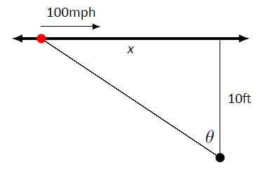
A camera is placed on a tripod 10ft from the side of a road. The camera is to turn to track a car that is to drive by at 100mph for a promotional video. The video's planners want to know what kind of motor the tripod should be equipped with in order to properly track the car as it passes by. Figure \(\PageIndex{2}\) shows the proposed setup.

Figure \(\PageIndex{2}\): Tracking a speeding car (at left) with a rotating camera.

How fast must the camera be able to turn to track the car?

Solution

We seek information about how fast the camera is to turn; therefore, we need an equation that will relate an angle \(\theta\) to the position of the camera and the speed and position of the car.

Figure \(\PageIndex{2}\) suggests we use a trigonometric equation. Letting \(x\) represent the distance the car is from the point on the road directly in front of the camera, we have

\[ \tan \theta = \frac{x}{10}\]

As the car is moving at 100mph, we have \(\frac{dx}{dt} = -100\)mph (as in the last example, since \(x\) is getting smaller as the car travels, \(\frac{dx}{dt}\) is negative). We need to convert the measurements so they use the same units; rewrite -100mph in terms of ft/s:

$$\frac{dx}{dt} = -100\frac{\text{m}}{\text{hr}} = -100\frac{\text{m}}{\text{hr}}\cdot5280\frac{\text{ft}}{\text{m}}\cdot\frac{1}{3600}\frac{\text{hr}}{\text{s}} =-146.\overline{6}\text{ft/s}.\]

Now take the derivative of both sides of Equation \(\PageIndex{9}\) using implicit differentiation:

\[\begin{align} \tan \theta &= \frac{x}{10} \\ \frac{d}{dt}\big(\tan \theta\big) &= \frac{d}{dt}\left(\frac{x}{10}\right) \\ \sec^2\theta\,\frac{d\theta}{dt} &= \frac{1}{10}\frac{dx}{dt}\\ \frac{d\theta}{dt} &= \frac{\cos^2\theta}{10}\frac{dx}{dt} \end{align}\]

We want to know the fastest the camera has to turn. Common sense tells us this is when the car is directly in front of the camera (i.e., when \(\theta = 0\)). Our mathematics bears this out. In Equation \(\PageIndex{14}\) we see this is when \(\cos^2\theta\) is largest; this is when \(\cos \theta = 1\), or when \(\theta = 0\).

With \(\frac{dx}{dt} \approx -146.67\)ft/s, we have

$$\frac{d\theta}{dt} = -\frac{1\text{rad}}{10\text{ft}}146.67\text{ft/s} = -14.667\text{radians/s}.\]

We find that \(\frac{d\theta}{dt}\) is negative; this matches our diagram in Figure \(\PageIndex{2}\) for \(\theta\) is getting smaller as the car approaches the camera.

What is the practical meaning of \(-14.667\) radians/s? Recall that 1 circular revolution goes through \(2\pi\) radians, thus \(14.667\) rad/s means \(14.667/(2\pi)\approx 2.33\) revolutions per second. The negative sign indicates the camera is rotating in a clockwise fashion.

We introduced the derivative as a function that gives the slopes of tangent lines of functions. This chapter emphasizes using the derivative in other ways. Newton's Method uses the derivative to approximate roots of functions; this section stresses the "rate of change" aspect of the derivative to find a relationship between the rates of change of two related quantities. In the next section we use Extreme Value concepts to optimize quantities.

Contributors and Attributions

• Gregory Hartman (Virginia Military Institute). Contributions were made by Troy Siemers and Dimplekumar Chalishajar of VMI and Brian Heinold of Mount Saint Mary's University. This content is copyrighted by a Creative Commons Attribution - Noncommercial (BY-NC) License. http://www.apexcalculus.com/

• Integrated by Justin Marshall.