3.1: The Geometric View - Zooming into the Graph of a Function

Learning Objectives

1. Describe the link between the local behavior of a function (seen by zooming into the graph) at a point and the tangent line to the graph of the function at that point.
2. Sketch a function’s derivative given its graph.

Locally, the graph of a function looks like a straight line

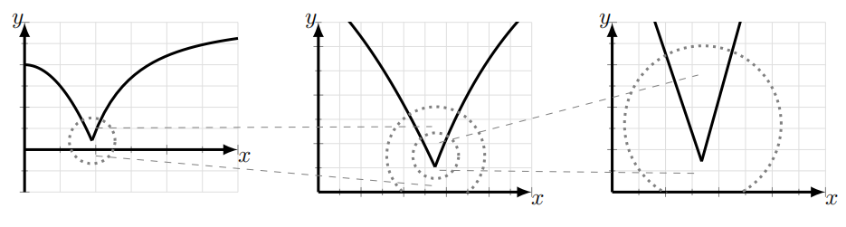
In this section we consider well-behaved functions whose graphs are "smooth", as opposed to the discrete data points of Chapter 2. We link the derivative to the local shape of the graph of the function. By local behavior we mean the shape we see when we zoom into a point on the graph. Imagine using a microscope where the center of the field of vision is some point of interest. As we zoom in, the graph looks flatter, until we observe a straight line, as shown in Figure 3.1.

Definition 3.1: Tangent line

The straight line that we see when we zoom into the graph of a smooth function at some point \(x_{0}\) is called the tangent line at \(x_{0}\).

Definition 3.2: Geometric definition of the derivative

The slope of the tangent line at the point \(x\) is denoted as the derivative of the function at the

Mastered Material Check

1. Write down the equation of a generic straight line.
2. Identify the slope of that straight line.
3. How many zeros does the function \(f(x)=x^{3}-x\) have? given point.

Figure 3.1: Zooming in on the graph of y = f(x) = x³−x at the point x = 1.5 makes the graph “look like” a straight line - the tangent line. The slope of that tangent line is the derivative of the function at x = 1.5.

Example 3.1 (Zooming into a polynomial)

Consider the function shown in Figure 3.1, \(y=f(x)=x^{3}-x\), and the point \(x=1.5\). Find the tangent line to the graph of this function by zooming in at the given point.

Solution

The graph of the function is shown in each panel of Figure 3.1, where we have indicated the point of interest with a red dot. Now zooming in on the given point. Locally, the graph resembles a straight line. This is the tangent line to \(f(x)\) at \(x=1.5\).

Example 3.2 (Zooming into the sine graph at the origin)

Determine the derivative of the function \(y=\sin (x)\) at \(x=0\) by zooming into the origin on its graph. Write down the equation of the tangent line at that point.

Solution

In Figure \(3.2\) we zoom into \(x=0\) on the graph of the function

\[y=\sin (x) . \nonumber \]

The sequence of zooms leads to a straight line (far right panel) that we identify once more as the tangent line to the function at \(x=0\). From the graph, the slope of this tangent line is 1 . We say that the derivative of the function \(y=f(x)=\sin (x)\) at \(x=0\) is 1 , and write \(f^{\prime}(0)=1\) to denote this. As this line goes through \((0,0)\) and has slope 1 , its equation is \(y=x\). We can also say that close to \(x=0\) the graph of \(y=\sin (x)\) looks a lot like the line \(y=x\).

Mastered Material Check

4. Using the far right panel of Figure 3.2, perform the calculations that verify the \(y=\sin (x)\) looks a lot like \(y=x\) near \(x=0\).
5. Give an example of a function with a discontinuity.

Figure 3.2: Zooming into the graph of the function \(y=f(x)=\sin (x)\) at the point \(x=0\). Eventually, the graph resembles a line of slope 1 . This is the tangent line at \(x=0\) and its slope, the derivative of \(y=\sin (x)\) at \(x=0\) is 1.

At a cusp or a discontinuity, the derivative is not defined

If we zoom into a function at a cusp or a discontinuity, there is no single straight line that describes the local behavior. For example, in Figure 3.3, we see two distinct lines meeting at a sharp "corner".

Figure 3.3: A function has no tangent line at a a cusp and the derivative is not defined at that point.

Zooming into a discontinuity presents another problem: there is no line at all, as in Figure 3.4. Finally, a function like \(1 / x\) has a singularity at \(x=0\) which shows up as a vertical line whose slope is infinite. In all such cases, we say that the function has no tangent line its derivative is not defined at the cusp, discontinuity, or singularity point.

Figure 3.4: Zooming into a function at a discontinuity shows no single distinct line that might be a tangent line.

From a Function to a Sketch of its Derivative

The tangent line to the graph of a function varies from point to point along the graph of the function - what we see when zooming in depends on the location of the zoom. This means that the derivative \(f^{\prime}(x)\) is, itself, also a function. Here we consider the connection between these two functions by using the graph of one to sketch the graph of other. The hand-sketch is approximate, but preserves important elements.

Example 3.3

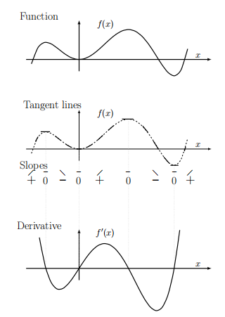
Consider the function in Figure 3.5. Reason about the tangent lines at various points along to sketch the derivative \(f^{\prime}(x)\).

Figure 3.5: The graph of a function. We sketch its derivative.

Solution

In Figure \(3.6\) we first sketch a few tangent lines along the graph of \(f(x)\). Focus on the slopes (rather than height, length, or other properties) of the dashes. Copying these lines in a row below the graph, we estimate their slopes roughly (approximate numerical values shown).

Figure 3.6: A few tangent lines of a function.

By convention, we "read" a graph from left to right. Slopes in Figure \(3.6\) are first positive, then zero, then negative, increase again through zero, and then positive. There are two locations with zero slope (horizontal dashes). Next, in Figure 3.7, we these rough values for slopes. Only a few points have been plotted for \(f^{\prime}(x)\), but these trends are clear: the derivative function has two zeros, and it dips below the axis between these places. In Figure \(3.7\) we emphasize how the original function lines up with its derivative \(f^{\prime}(x)\).

Figure 3.7: Sketching the derivative of a function.

We have aligned these graphs so that the slope of \(f(x)\) matches the value of \(f^{\prime}(x)\) shown directly below.

Example 3.4

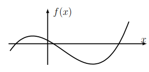
Sketch the derivative of the function shown in Figure 3.8.

Figure 3.8: In Example 3.4, we sketch the derivative of this function.

Solution

We can get a good rough sketch by simply noting where the slopes are positive, negative, or zero. See Figure \(3.9\) for the entire process. The thin vertical lines demonstrate that \(f^{\prime}(x)=0\) coincides with tops of hills or bottom of valleys on the graph of the function \(f(x)\).

Figure 3.9: Sketching the derivative of a function for Example \(3.4\)

Mastered Material Check

6. Sketch the "zooming in" graph of the function \(y=f(x)=\sin (x)\) at \(x=1\).
7. How many local minima are depicted in Figure 3.5?

Constant and linear functions and their derivatives

Example 3.5: Derivative of \(y=C\)

Use a geometric argument to determine the derivative of the function \(y=f(x)=C\) at any point \(x_{0}\) on its graph.

Solution

This function is a horizontal straight line, whose slope is zero everywhere. Thus "zooming in" at any point \(x\), leads to the same result, so the derivative is 0 everywhere.

Example 3.6: Derivative of \(y=B x\)

Use a geometric argument to determine the derivative of the function \(y=f(x)=B x\) at any point \(x_{0}\) on its graph.

Solution

The function \(y=B x\) is a straight line of slope \(B\). At any point on its graph, it has the same slope, \(B\). Thus the derivative is equal to \(B\) at any point on the graph of this function.

Notice that in the above two examples we have found the derivative for the two power functions, \(y=x^{0}\) and \(y=x^{1}\). We summarize:

The derivative of any constant function is zero. The derivative of the function \(y=x\) is 1 . The derivative of the function \(y=k \cdot x\) is \(k\).

Molecular Motors

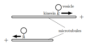
Microtubules (MT) are long, rod-like cellular structures (introduced in Chapter 2) with both structural and transportation roles in living cells. Human nerve cells can be up to 1 meter in length, which makes for a challenge to move material from the cell body - where it is made - to the cell ends where it is needed for repair or metabolism. Microtubules act like highways for "molecular motors", proteins that "drive" along these routes, transporting the necessary cargo.

Microtubules have distinct ends (called "plus" and "minus" ends). Some motors specialize in moving towards the + end, while others move towards the - end. Figure \(3.10\) is a schematic diagram of kinesin (represented by the letter \(k\) ), a plus-end directed motor. As shown in the figure, kinesin can hop off one MT and onto another MT pointing in the opposite direction.

Figure 3.10: The molecular motor kinesin walks towards a microtubule "plus" end. It can detach and reattach to another microtubule.

In Example 3.7, we study a sample vesicle track (displacement, \(y\) over time \(t\) ) and decipher the sequence of motor events that caused that motion.

Example 3.7: Motion of molecular motors

The displacement \(y(t)\) of a vesicle is shown in Figure 3.10(a).

(a) Sketch the corresponding instantaneous velocity \(v(t)\) for the vesicle.

(b) Use your sketch to explain what was happening to the kinesin carrying that vesicle.

Figure 3.11: Molecular motors: (a) The displacement of the vesicle. (b) The velocity of the vesicle.

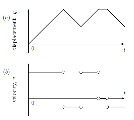
Solution

(a) The plot in Figure 3.11(a) consists of straight line segments with sharp corners (cusps). Over each of these line segments, the slope \(d y / d t\) (which corresponds to the instantaneous velocity, \(v(t))\) is constant. Segments with positive slope correspond to motion towards the right (as in the top microtubule track in Figure 3.10. Over times where the slope is negative, the motion is to the left. Where the slope is zero (flat graph), the vesicle was stationary.

In Figure 3.11(b), we sketch the graph of the instantaneous velocity, \(v(t)\). Observe that \(v(t)\), which is the derivative of \(y(t)\), is not defined at the points where \(y(t)\) has "corners".

(b) Based on Figure 3.11(b), the kinesin motor was moving on a right-facing microtubule, then hopped onto a left-facing microtubule, and then hopped back to a right -facing microtubule. For a brief time it was either stuck or detached from the microtubule tracks (stationary part). Finally, it hopped onto a left-moving microtubule.

Mastered Material Check

8. If the equation of the tangent line to \(f(x)\) at \(x=1\) is \(y=m x+b\), what is \(f^{\prime}(1)\) ?
9. Sketch the graph of the derivative of the function \(y=C\). (What slope do you see at each point when you "zoom in"?