3.2: The Analytic View - Calculating the Derivative

Learning Objectives

1. Explain the definition of a continuous function.
2. Identify functions with various types of discontinuities.
3. Evaluate simple limits of rational functions.
4. Calculate the derivative of a simple function using the definition of the derivative, \(2.7\).

Technical matters: continuous functions and limits

In Chapter 2, we saw functions made up of discrete data points. In Chapter 1 we studied several continuous functions: power, polynomial or rational. Intuitively, on the graph of a continuous function, every point is connected to neighbouring points. For example, the power function Equation (2.1), \(y(t)=c t^{2}\) is continuous for all values of \(t\), whereas a function such as \(y=\sqrt{x}\) is continuous and defined as a real number only for \(x \geq 0\). The function \(y=1 /(x+1)\) is defined and continuous for \(x \neq-1\) (since division by zero is undefined).

We now make the intuitive discussion more precise with a formal definition, based on the concept of a limit. We first define what it means for a function to be continuous, and then show how limits are computed to test that definition.

Definition 3.3: Contimuous function

We say that \(y=f(x)\) is continuous at a point \(x=a\) in its domain if

\[\lim _{x \rightarrow a} f(x)=f(a) . \nonumber \]

By this we mean that the function is defined at \(x=a\), that the above limit exists, and that it matches with the value that the function takes at the given point.

This definition has two important parts. First, the function should be defined at the point of interest, and second, the value assigned by the function has to "fit the local behavior" in the sense of the limit. This rules out a "jump" or "break" in the graph. When the above is not true at some point \(x_{s}\), we say that the function is discontinuous at \(x_{s}\). We give a few examples to demonstrate some different types of discontinuities that exist. At the same time we illustrate how limits are calculated.

Function with a hole in its graph. Consider a function of the form

\[f(x)=\frac{(x-a)^{2}}{(x-a)} . \nonumber \]

Then if \(x \neq a\), we can cancel a common factor, and obtain \((x-a)\). At \(x=a\), the function is not defined because \(\left(\frac{0}{0}\right)\) - which is undefined - results. In short, we have

\[f(x)=\frac{(x-a)^{2}}{(x-a)}= \begin{cases}x-a & x \neq a \\ \text { undefined } & x=a .\end{cases} \nonumber \]

Even though the function is not defined at \(x=a\), we can still evaluate the limit of \(f\) as \(x\) approaches \(a\). We write

\[\lim _{x \rightarrow a} f(x)=\lim _{x \rightarrow a} \frac{(x-a)^{2}}{(x-a)}=\lim _{x \rightarrow a} x-a=0, \nonumber \]

and say that "the limit as \(x\) approaches \(a\) " exists and is equal to 0 . We also say that the function has a removable discontinuity. If we add the point \((a, 0)\) to the set of points at which the function is defined then we obtain a continuous function identical to the function \(x-a\). See also Appendix D.

Function with jump discontinuity. Consider the function

\[f(x)= \begin{cases}-1 & x \leq a \\ 1 & x>a\end{cases} \nonumber \]

We say that the function has a jump discontinuity at \(x=a\). As we approach the point of discontinuity we observe that the function has two distinct values, depending on the direction of approach. We formally capture this observation using right and left hand limits,

\[\lim _{x \rightarrow a-} f(x)=-1, \quad \lim _{x \rightarrow a+} f(x)=1 . \nonumber \]

Notice we use \(\lim _{x \rightarrow a-}\) to denote approaching \(a\) from the left, and \(\lim _{x \rightarrow a+}\) to denote approaching \(a\) from the right. Since the left and right limits are unequal, we say that "the limit does not exist" (abbreviated DNE).

Function with blow up discontinuity. Consider the function

\[f(x)=\frac{1}{x-a} . \nonumber \]

Then as \(x\) approaches \(a\), the denominator approaches 0 , and the value of the function goes to \(\pm \infty\). We say that the function "blows up" at \(x=a\) and that the limit, \(\lim _{x \rightarrow a} f(x)\), does not exist.

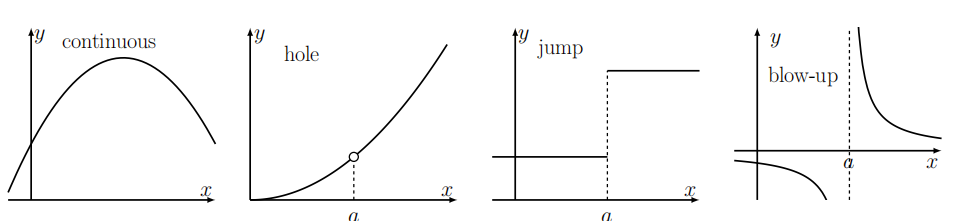
Figure 3.12 illustrates the differences between functions that are continuous everywhere, those that have a hole in their graph, and those that have a jump discontinuity or a blow up at some point \(a\).

Examples of limits. We now examine several examples of computations of limits. More details about properties of limits are provided in Appendix D.

By Definition 3.3, to calculate the limit of any function at a point of continuity, we simply evaluate the function at the given point.

Figure 3.12: Left to right: a continuous function, a function with a removable discontinuity, a jump discontinuity, and a function with blow up discontinuity.

Mastered Material Check

11. Sketch the graph of the function \(f(x)=\frac{(x-1)^{2}}{(x-1)}\).
12. What type of discontinuity does \(\frac{x^{2}+4 x+4}{x+2}\) have?
13. What type of discontinuity does \(\frac{x^{2}+4 x+4}{x+4}\) have?

Example 3.8 (Simple limit of a continuous function)

Find the following limits:

(a) \(\lim _{x \rightarrow 3} x^{2}+2\) (b) \(\lim _{x \rightarrow 1} \frac{1}{x+1}\) (c) \(\lim _{x \rightarrow 10} \frac{x}{1+x}\).

Solution

In each case, the function is continuous at the point of interest (at \(x=3,1,10\), respectively). Thus, we simply "plug in" the values of \(x\) in each case to obtain

(a) \(\lim _{x \rightarrow 3} x^{2}+2=3^{2}+2=11\) (b) \(\lim _{x \rightarrow 1} \frac{1}{x+1}=\frac{1}{2}\) (c) \(\lim _{x \rightarrow 10} \frac{x}{1+x}=\frac{10}{11}\).

Example 3.9 (Hole in graph limits)

Calculate the limits of the following functions. Note that each has a removable discontinuity (" a hole in its graph").

(a) \(\lim _{x \rightarrow 3} \frac{x^{2}-6 x+9}{x-3}\) (b) \(\lim _{x \rightarrow-1} \frac{x^{2}+3 x+2}{x+1}\).

Solution

We first simplify algebraically by factoring the numerator, and then evaluate the limit. Note that the simplification is possible so long as we evaluate the limit, rather than the actual function, at the point of discontinuity.

(a) \(\lim _{x \rightarrow 3} \frac{x^{2}-6 x+9}{x-3}=\lim _{x \rightarrow 3} \frac{(x-3)^{2}}{(x-3)}=\lim _{x \rightarrow 3}(x-3)=0\).

(b) \(\lim _{x \rightarrow-1} \frac{x^{2}+3 x+2}{x+1}=\lim _{x \rightarrow-1} \frac{(x+1)(x+2)}{(x+1)}=\lim _{x \rightarrow-1}(x+2)=1\).

Example 3.10

(Limit involving \(\sin (x)\) ) Use the observation made in Example \(3.2\) to arrive at the value of \(\lim _{x \rightarrow 0} \frac{\sin (x)}{x}\).

Solution

Example \(3.2\) illustrated the fact that close to \(x=0\) the function \(\sin (x)\) has the following behavior:

\[\sin (x) \approx x, \quad \text { or } \quad \frac{\sin (x)}{x} \approx 1 . \nonumber \]

This is equivalent to the result

\[\lim _{x \rightarrow 0} \frac{\sin (x)}{x}=1 . \nonumber \]

We read this "as \(x\) approaches zero, the limit of \(\sin (x) / x\) is 1 ." This limit is used in later calculations involving derivatives of trigonometric functions.

Mastered Material Check

14. How do these examples change if the limit approaches a different value of \(x\) ?

Computing the derivative

As discussed in Section 2.5, calculating a derivative requires the use of limits. To summarize:

1. For the secant line connecting the points \(x\) and \(x+h\) on the graph of a function, in the limit \(h \rightarrow 0\), those points get closer together, leading to a tangent line.
2. The slope of a secant line is an average rate of change, but in the limit ( \(h \rightarrow 0\) ), we obtain the derivative, which is the slope of the tangent line.

We illustrate how to use the definition of the derivative to compute a few derivatives.

Example 3.11

(Derivative of a linear function) Using Definition \(2.7\) of the derivative, compute the derivative of the function \(y=f(x)=B x+C\).

Solution

We have already used a geometric approach to find the derivative of related functions in Examples 3.5-3.6. Here we do the formal calculation as follows:

\[\begin{array}{rlr} f^{\prime}(x) & =\lim _{h \rightarrow 0} \frac{f(x+h)-f(x)}{h} & \text { (start with the definition) } \\ & =\lim _{h \rightarrow 0} \frac{[B(x+h)+C]-[B x+C]}{h} & \text { (apply it to the function) } \\ & =\lim _{h \rightarrow 0} \frac{B x+B h+C-B x-C}{h} & \text { (expand the numerator) } \\ & =\lim _{h \rightarrow 0} \frac{B h}{h} & \text { (simplify) } \\ & =\lim _{h \rightarrow 0} B & \text { (cancel a factor of } h \text { ) } \\ & =B & \text { (evaluate the limit). } \end{array} \nonumber \]

Hence, we confirmed that the derivative of \(f(x)=B x+C\) is \(f^{\prime}(x)=B\). This agrees with the sum of the derivatives of the two parts, \(B x\) and \(C\) found in Examples 3.5-3.6. (Indeed, as we establish shortly, the derivative of the sum of two functions is the same as the sum of their derivatives.)

Mastered Material Check

15. What other notations express the derivative of \(f(x)\) ?

Example 3.12 (Derivative of the cubic power function)

Compute the derivative of the function \(y=f(x)=K x^{3}\).

Solution

For \(y=f(x)=K x^{3}\) we have

\[\begin{aligned} \frac{d y}{d x} & =\lim _{h \rightarrow 0} \frac{f(x+h)-f(x)}{h} \\ & =\lim _{h \rightarrow 0} \frac{K(x+h)^{3}-K x^{3}}{h} \\ & =\lim _{h \rightarrow 0} K \frac{\left(x^{3}+3 x^{2} h+3 x h^{2}+h^{3}\right)-x^{3}}{h} \\ & =\lim _{h \rightarrow 0} K \frac{\left(3 x^{2} h+3 x h^{2}+h^{3}\right)}{h} \\ & =\lim _{h \rightarrow 0} K\left(3 x^{2}+3 x h+h^{2}\right) \\ & =K\left(3 x^{2}\right)=3 K x^{2} . \end{aligned} \nonumber \]

Thus the derivative of \(f(x)=K x^{3}\) is \(f^{\prime}(x)=3 K x^{2}\).

Example 3.13

Use the definition of the derivative to compute \(f^{\prime}(x)\) for the function \(y=f(x)=1 / x\) at the point \(x=1\).

Solution

We write down the formula for this calculation at any point \(x\) and then simplify algebraically, using common denominators to combine fractions, and then, in the final step, calculate the limit formally. Lastly we substitute the value \(x=1\) to find \(f^{\prime}(1)\).

\[\begin{array}{rrr} f^{\prime}(x) & =\lim _{h \rightarrow 0} \frac{f(x+h)-f(x)}{h} & \text { (the definition) } \\ & =\lim _{h \rightarrow 0} \frac{\frac{1}{(x+h)}-\frac{1}{x}}{h} & \text { (applied to the function) } \\ & =\lim _{h \rightarrow 0} \frac{\frac{[x-(x+h)]}{x(x+h)}}{h} & \text { (common denominator) } \\ & =\lim _{h \rightarrow 0} \frac{-h}{h x(x+h)} & \text { (algebraic simplification) } \\ & =\lim _{h \rightarrow 0} \frac{-1}{x(x+h)} & \text { (cancel factor of } h \text { ) } \\ & =-\frac{1}{x^{2}} & \text { (limit evaluated) } \end{array} \nonumber \]

Thus, the derivative of \(f(x)=1 / x\) is \(f^{\prime}(x)=-1 / x^{2}\) and at the point \(x=1\) it takes the value \(f^{\prime}(1)=-1\).

In Exercise 3.8 we apply similar techniques to the derivative of the squareroot function to show that

\[y=f(x)=\sqrt{x} \quad \Rightarrow \quad f^{\prime}(x)=\frac{1}{2 \sqrt{x}} . \nonumber \]

In the next chapter, we formalize some observations about derivatives of power functions and rules of differentiation. This allows us to simplify some of the calculations involved in finding derivatives. W See the steps in a related calculation of the derivative of \(y=f(x)=K x^{n}\).

See the calculation of the derivative of \(y=f(x)=1/x\).