
3.3: The Computational View - Software to the Rescue!
- Page ID
- 121096

\( \newcommand{\vecs}[1]{\overset { \scriptstyle \rightharpoonup} {\mathbf{#1}} } \)
\( \newcommand{\vecd}[1]{\overset{-\!-\!\rightharpoonup}{\vphantom{a}\smash {#1}}} \)
\( \newcommand{\id}{\mathrm{id}}\) \( \newcommand{\Span}{\mathrm{span}}\)
( \newcommand{\kernel}{\mathrm{null}\,}\) \( \newcommand{\range}{\mathrm{range}\,}\)
\( \newcommand{\RealPart}{\mathrm{Re}}\) \( \newcommand{\ImaginaryPart}{\mathrm{Im}}\)
\( \newcommand{\Argument}{\mathrm{Arg}}\) \( \newcommand{\norm}[1]{\| #1 \|}\)
\( \newcommand{\inner}[2]{\langle #1, #2 \rangle}\)
\( \newcommand{\Span}{\mathrm{span}}\)
\( \newcommand{\id}{\mathrm{id}}\)
\( \newcommand{\Span}{\mathrm{span}}\)
\( \newcommand{\kernel}{\mathrm{null}\,}\)
\( \newcommand{\range}{\mathrm{range}\,}\)
\( \newcommand{\RealPart}{\mathrm{Re}}\)
\( \newcommand{\ImaginaryPart}{\mathrm{Im}}\)
\( \newcommand{\Argument}{\mathrm{Arg}}\)
\( \newcommand{\norm}[1]{\| #1 \|}\)
\( \newcommand{\inner}[2]{\langle #1, #2 \rangle}\)
\( \newcommand{\Span}{\mathrm{span}}\) \( \newcommand{\AA}{\unicode[.8,0]{x212B}}\)
\( \newcommand{\vectorA}[1]{\vec{#1}} % arrow\)
\( \newcommand{\vectorAt}[1]{\vec{\text{#1}}} % arrow\)
\( \newcommand{\vectorB}[1]{\overset { \scriptstyle \rightharpoonup} {\mathbf{#1}} } \)
\( \newcommand{\vectorC}[1]{\textbf{#1}} \)
\( \newcommand{\vectorD}[1]{\overrightarrow{#1}} \)
\( \newcommand{\vectorDt}[1]{\overrightarrow{\text{#1}}} \)
\( \newcommand{\vectE}[1]{\overset{-\!-\!\rightharpoonup}{\vphantom{a}\smash{\mathbf {#1}}}} \)
\( \newcommand{\vecs}[1]{\overset { \scriptstyle \rightharpoonup} {\mathbf{#1}} } \)
\( \newcommand{\vecd}[1]{\overset{-\!-\!\rightharpoonup}{\vphantom{a}\smash {#1}}} \)
- Use software to numerically compute an approximation to the derivative.
- Explain that the approximation replaces a (true) tangent line with an (approximating) secant line.
- Explain using words how the derivative shape is connected with the shape of the original function.
- Interpret the differences between two types of biochemical kinetics: Michaelis-Menten and Hill function.
We have explored geometric and analytic aspects of the derivative. Here we show a third aspect of the derivative: its numerical implementation using a simple spreadsheet. The ideas introduced here reappear in a variety of problems where repetitive calculations are needed to arrive at a solution.
A numerical derivative is an approximation to the value of the derivative, obtained by using a finite value of \(\Delta x\),
\[f^{\prime}(x)_{\text {numerical }} \approx \frac{\Delta f}{\Delta x} \quad \text { rather than the actual value } f^{\prime}(x)_{\text {actual }}=\lim _{\Delta x \rightarrow 0} \frac{\Delta f}{\Delta x} . \nonumber \]
The numerical derivative would be a good approximation of the true derivative provided that \(\Delta x\) is "small enough", that is, a step size for which the function \(f(x)\) does not changes dramatically. Since \(\Delta f\) is the difference of two values of \(f,(\Delta f=f(x+\Delta x)-f(x))\) it follows that the numerical derivative is the same as the slope of a secant line. This important realization, associated with the second learning goal in this section, means that a secant line is often used to approximate a tangent line, and the slope of a secant line is used to approximate a derivative in numerical computations. We see this idea again in several contexts.
Derivative of Michaelis-Menten and Hill functions
A spreadsheet can be used to numerically approximate derivatives. We illustrate this using as examples the reaction speeds for Michaelis-Menten Equation (1.8) and Hill function kinetics, Equation (1.7) (see Section 1.5), repeated below:
\[\begin{gathered} v_{M M}=f_{1}(c)=\frac{K c}{a+c}, \\ v_{H i l l}=f_{2}(c)=\frac{K c^{n}}{a^{n}+c^{n}} . \end{gathered} \nonumber \]
- Describe how to find the derivative of a function \(f(x)\) at \(x=x_{0}\) analytically.
- Describe how to find the derivative of a function \(f(x)\) at \(x=x_{1}\) geometrically. (Both \(f_{1}(c), f_{2}(c)\) are shown as functions of \(c\) in Figure 3.13a.) Our goal is to use a spreadsheet to compute a numerical approximation of the derivative of these two reaction speeds with respect to the chemical concentration \(c\).
Featured Problem 3.1 (The derivative on a spreadsheet): Use a spreadsheet (or your favorite software) to plot the derivatives of the functions \(v_{M M}=f_{1}(c), v_{H i l l}=f_{2}(c)\).
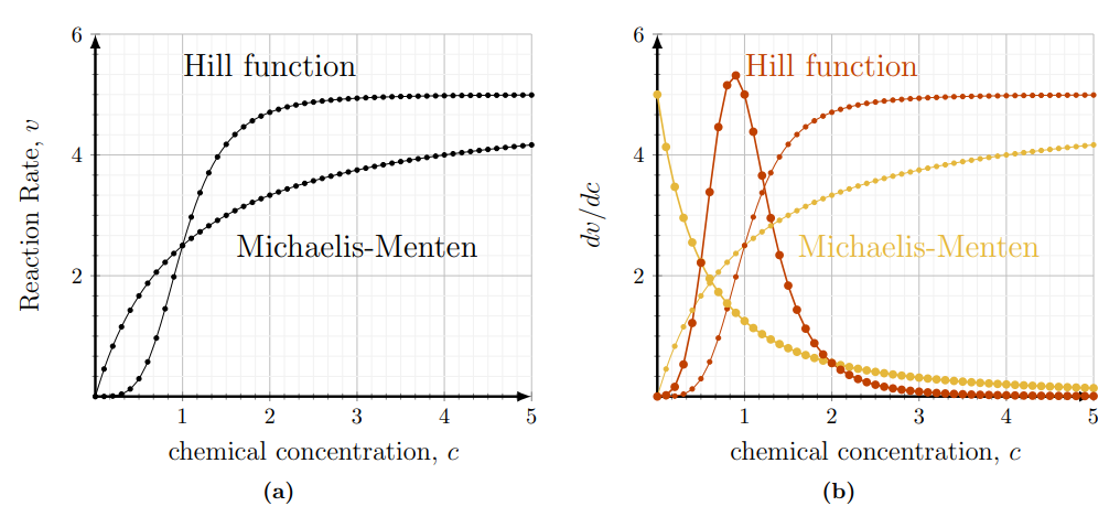
Solution. Figure 3.13 shows the results of the spreadsheet calculation, but here we use only the Hill function to demonstrate typical spreadsheet manipulations.
(A) Open your favorite spreadsheet and label columns where data will be kept. In the link we display a spreadsheet with columns for the step size \(\Delta c\), concentration \(c\), and values of the function \(f_{2}(c)\), with \(K=5, a=1, n=4\). The last column contains the approximation for the derivative \(\Delta f / \Delta c\).
(1) We input the desired step size \(\Delta c\), here set to \(0.1\) (cell A2)
(2) Input the value of \(c\) at which to start the calculations. Here we used \(c=0\) as the left endpoint (input 0 into cell \(\mathbf{B 2}\) ). Then let the spreadsheet create the entire set of \(c\) values by inputting \(=B 2+\$ A \$ 2\) in cell \(\mathbf{B} 3\), and dragging the "fill handle" (small square dot on bottom right hand corner) down the column. Note that the symbols \(\$\) are universally used in spreadsheets to denote an absolute reference to a particular cell, whereas all other references are relative.
(3) In cell C2 type \(=5 * B 2 \wedge 4 /(1+B 2 \wedge 4)\) to create the formula for the desired function. The symbol \(\wedge\) denotes a power. This will generate the Figure 3.13: (a) A plot of \(f_{1}(c), f_{2}(c)\) produced on a spreadsheet. (b) A plot of both the functions and their (approximate) derivatives.
Link to Google Sheets. This spreadsheet shows how to create an approximation for the derivative of the Hill function in (3.7). Fig 3.13 was produced by a similar set of calculations, see Feature Problem 3.1. You can view this sheet and copy it elsewhere. You cannot edit it as is. first point on the graph to be plotted. Similarly drag the fill handle to generate the rest of the points \(f_{2}(c)\) corresponding to the all \(c\) values.
(B) Next, we compute the desired numerical approximations of the derivatives.
(1) Use column \(\mathbf{D}\) for the numerical derivative of \(f_{2}(c)\). To do so, approximate the actual derivative with a finite difference,
\[\frac{\Delta f_{2}}{\Delta c} \approx \frac{d f_{2}}{d c} . \nonumber \]
Note: importantly, the two expressions are not equal. However, for sufficiently small \(\Delta c\), they approximate one another well.
(2) Dragging the fill handle down the column generates the desired list of values of the numerical derivative.
(C) Create a chart and plot the results. The \(x\) axis is the set of values of \(c\).
Results of the above process (but modified for the two functions and their two derivatives) lead to the graphs shown on the right panel of Figure 3.13.
Interpret the graphs of the derivatives in Figure 3.13b in terms of the way that reaction speed increases as the chemical concentration is increased in each of Michaelis-Menten and Hill function kinetics
Solution
Both derivatives are positive everywhere, since both \(f_{1}(c)\) and \(f_{2}(c)\) are increasing functions. For Michaelis-Menten, the derivative is always decreasing. This agrees with the observation that \(f_{1}(c)\) (thin yellow curve) gradually levels off and flattens as \(c\) increases. While the reaction rate \(v_{M M}\) increases with \(c\), the rate of increase, \(d v / d c\), slows due to saturation at higher \(c\) values.
18. Given time dependent data, can an exact derivative ever be determined?
In contrast, the Hill function derivative starts at zero, increases sharply, and only then decreases to zero. Correspondingly, the Hill function (thin red curve) is flat at first, then becomes steeply increasing, and finally flattens to an asymptote. We can summarize this biochemically by saying that the initial reaction rate \(v_{\text {Hill }}\) is small and hardly changes near \(c \sim 0\). For intermediate range of \(c\), the reaction rate depends sensitively on \(c\) (evidenced by large \(d v / d c\). . As \(c\) increases to higher values, saturation slows down the rate of reaction, leading to the drop in \(d v / d c\).