3.5: Exercises

3.1. Sketching the derivative (geometric view). Shown in Figure 3.14 are four functions. Sketch the derivative of each of these functions.

Figure 3.14: Figure for Exercise 3.1; graphs of four different functions.

3.2. Sketching the function given its derivative. Given the information in Table \(3.2\) about the the values of the derivative of a function, \(g(x)\), sketch a (very rough) graph the function for \(-3 \leq x \leq 3\).

Table 3.2: Derivative data for two different functions: \(g^{\prime}(x)\) (Exercise 3.2) and \(f^{\prime}(x)\) (Exercise 3.3).

\(x\)	\(g^{\prime}(x)\)	\(f^{\prime}(x)\)
-3	-1	0
-2	0	+
-1	2	0
0	1	-
1	0	0
2	-1	+
3	-2	0

3.3. What the sign of the derivative tells us. Given the information about the signs of the derivative of a function, \(f(x)\) found in Table 3.2, sketch a (very rough) graph of the function for \(-3 \leq x \leq 3\).

3.4. Shallower or steeper rise. Shown in Figure 3.15 are two similar functions, both increasing from 0 to 1 but at distinct rates. Sketch the derivatives of each one. Then comment on what your sketch would look like for a discontinuous "step function", defined as follows:

\[f(x)= \begin{cases}0 & x<0 \\ 1 & x \geq 0 .\end{cases} \nonumber \]

Figure 3.15: Figure for Exercise 4; two similar functions increasing at distinct rates.

3.5. Introduction to velocity and acceleration. The acceleration of a particle is the derivative of its velocity. Shown in Figure 3.16 is the graph of the velocity of a particle moving in one dimension. Indicate directly on the graph any time(s) at which the particle’s acceleration is zero.

Figure 3.16: Figure for Exercise 5; velocity of a particle moving in one direction.

3.6. Velocity, continued. The vertical height of a ball, \(d\) (in meters) at time \(t\) (seconds) after it was thrown upwards was found to satisfy \(d(t)=14.7 t-4.9 t^{2}\) for the first 3 seconds of its motion.

(a) What is the initial velocity of the ball (i.e. the instantaneous velocity at \(t=0)\) ?

(b) What is the instantaneous velocity of the ball at \(t=2\) seconds?

3.7. Geometric view, continued. Consider Figure 3.17.

Figure 3.17: Figures of functions and derivatives for Exercise 7.

(a) Given the function in Figure 3.17(a), graph its derivative.

(b) Given the function in Figure 3.17(b), graph its derivative

(c) Given the derivative \(f^{\prime}(x)\) shown in Figure 3.17(c) graph the function \(f(x)\).

(d) Given the derivative \(f^{\prime}(x)\) shown in Figure 3.17(d) graph the function \(f(x)\).

3.8. Computing the derivative of square-root (from the definition). Consider the function

\[y=f(x)=\sqrt{x} . \nonumber \]

(a) Use the definition of the derivative to calculate \(f^{\prime}(x)\). Consider using the following algebraic simplification:

\[\frac{(\sqrt{a}-\sqrt{b})(\sqrt{a}+\sqrt{b})}{(\sqrt{a}+\sqrt{b})}=\frac{a-b}{(\sqrt{a}+\sqrt{b})} . \nonumber \]

(b) Find the slope of the function at the point \(x=4\).

(c) Find the equation of the tangent line to the graph at this point.

3.9. Computing the derivative. Use the definition of the derivative to compute the derivative of the function \(y=f(x)=C /(x+a)\) where \(C\) and \(a\) are arbitrary constants. Show that your result is \(f^{\prime}(x)=-C /(x+\) \(a)^{2}\)

3.10. Computing the derivative. Consider the function

\[y=f(x)=\frac{x}{(x+a)} . \nonumber \]

(a) Show that this function can be written as \(f(x)=1-\frac{a}{(x+a)}\).

(b) Use the results of Exercise 9 to determine the derivative of this function (note: you do not need to use the definition of the derivative to do this computation). Show that you get \(f^{\prime}(x)=\frac{a}{(x+a)^{2}}\).

3.11. Molecular motors.

Figure 3.18: Figure for Exercise 3.11, molecular motors.

(a) Figure 3.18 (a) shows the displacement of a vesicle carried by a molecular motor. The motor can either walk right (R), left (L) along one of the microtubules or it can unbind (U) and be stationary, then rebind again to a microtubule. Sketch a rough graph of the velocity of the vesicle \(v(t)\) and explain the sequence of events (using the letters R, L, U) that resulted in this motion.

(b) Figure 3.18 (b) shows the velocity \(v(t)\) of another vesicle. Sketch a rough graph of its displacement starting from \(y(0)=0\).

3.12. Concentration gradient. Certain types of tissues - epithelia - are made up of thin sheets of cells. Substances are taken up on one side of the sheet by some active transport mechanism, and then diffuse down a concentration gradient by a mechanism called facilitated diffusion on the opposite side.

Figure 3.19: Figure for Exercise 3.12: concentration profile of a substance.

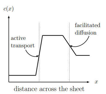
Shown in Figure 3.19 is the concentration profile \(c(x)\) of some substance across the width of the sheet ( \(x\) represents distance). Sketch the corresponding concentration gradient, i.e. sketch \(c^{\prime}(x)\), the derivative of the concentration with respect to \(x\).

3.13. Tangent line to a simple function. What is the slope of the tangent line to the function \(y=f(x)=5 x+2\) when \(x=2\) ? when \(x=4\) ? How would this slope change if a negative value of \(x\) was used? Why?

3.14. Slope of the tangent line. Use the definition of the derivative to compute the slope of the tangent line to the graph of the function \(y=\) \(3 t^{2}-t+2\) at the point \(t=1\).

3.15. Tangent line. Find the equation of the tangent line to the graph of \(y=f(x)=x^{3}-x\) at the point \(x=1.5\) shown in Figure 3.1. You may use the fact that the tangent line goes through \((1.7,1.47)\) as well as the point of tangency.

3.16. Numerically computed derivative. Consider the two Hill functions

\[H_{1}(x)=\frac{x^{2}}{0.01+x^{2}}, \quad H_{2}(x)=\frac{x^{4}}{0.01+x^{4}} \nonumber \]

(a) Sketch a rough graph of these two functions on the same plot and/or describe in words what the two graphs would look like.

(b) On a second plot, sketch a rough graph of both derivatives of these functions and/or describe in words what the two derivatives would look like.

(c) Using a spreadsheet or your favourite software, plot the two functions over the range \(0 \leq x \leq 1\).

(d) Use the spreadsheet to calculate an approximation for the derivatives \(H_{1}^{\prime}(x), H_{2}^{\prime}(x)\) and plot these two functions together.

Note: in order to have a reasonably accurate set of graphs, you must select a small step size of \(\Delta x \approx 0.01\).

3.17. More numerically computed derivatives. As we see in Chapter 14, trigonometric functions such as \(\sin (t)\) and \(\cos (t)\) can be used to describe biorhythms of various types. Here we numerically compute the first and second derivative of \(y=\sin (t)\) and show the relationships between the trigonometric functions and their derivatives. We use only numerical methods (e.g. a spreadsheet), but in Chapter 14, we also study the analytical calculation of the same derivatives.

(a) Use a spreadsheet (or your favourite software) to plot, on the same graph the two functions

\[y_{1}=\sin (t), y_{2}=\cos (t), \quad 0 \leq t \leq 2 \pi \approx 6.28 . \nonumber \]

Note that you should use a fairly small step size, e.g. \(\Delta t=0.01\) to get a reasonably accurate approximation of the derivatives.

(b) Use the same spreadsheet to (numerically) calculate (an approximate) derivative \(y_{1}^{\prime}(t)\) and add it to your graph.

(c) Now calculate \(y_{1}^{\prime \prime}(t)\), that is (an approximation to) the derivative of the derivative of the sine function and add this to your graph.