4.2: Application of the Second Derivative to Acceleration

Learning Objectives

1. Recognize that velocity and acceleration are first and second derivatives of position with respect to time (and that velocity and position are first and second antiderivatives of acceleration.)
2. Given constant acceleration, be able to find the velocity and displacement of the moving object.

We have already defined the "derivative of a derivative" as the second derivative. Here we provide a natural example of a second derivative, the acceleration of an object: the rate of change of the velocity (which is, as we have seen, the rate of change of a displacement). We restate these relationships in terms of antiderivatives below.

Position, velocity, and acceleration

Consider an object falling under the force of gravity. Let \(y(t)\) denote the position of the object at time \(t\). From now on, we refer to the instantaneous velocity at time \(t\) simply as the velocity, \(v(t)\).

Definition 4.1: (The Velocity)

Given the position of some particle as a function of time, \(y(t)\), we define the velocity as the rate of change of the position, i.e. the derivative of \(y(t)\) :

\[v(t)=\frac{d y}{d t}=y^{\prime}(t) . \nonumber \]

In general, \(v\) may depend on time, which we indicated by writing \(v(t)\).

Definition 4.2: (The Acceleration)

We define the acceleration as the (instantaneous) rate of change of the velocity, i.e. as the derivative of \(v(t)\).

\[a(t)=\frac{d v}{d t}=v^{\prime}(t) \nonumber \]

(acceleration could also depend on time, hence a \((t)\) ).

Mastered Material Check

12. Give three different examples of possible units for velocity.
13. Give three different examples of possible units for acceleration. Since the acceleration is the derivative of the derivative of the original function, we also use the notation

\[a(t)=\frac{d}{d t}\left(\frac{d y}{d t}\right)=\frac{d^{2} y}{d t^{2}}=y^{\prime \prime}(t) . \nonumber \]

Note: we have used three equivalent ways of writing a second derivative. This notation evolved for historical reasons, and is used interchangeably in science. Acceleration is a second derivative of the position.

Given \(a(t)\), the acceleration as a function of \(t\), we can use antidifferentiation to obtain the velocity \(v(t)\). Similarly, we can use the velocity \(v(t)\) to determine the position \(y(t)\) (up to some constant). The constants must be obtained from other information, as the next examples illustrate.

Example 4.10: (Uniformly accelerated motion of a falling object)

Suppose that the acceleration of an object is constant in time, i.e. \(a(t)=-g=\) constant. Use antidifferentiation to determine the velocity and the position of the object as functions of time.

Note: here we have a coordinate system in which the positive direction is "upwards", and so the acceleration, which is in the opposite direction, is negative. On Earth, \(g=9.8 \mathrm{~m} / \mathrm{s}^{2}\).

Solution

First, what function of time \(v(t)\) has the property that

\[a(t)=v^{\prime}(t)=-g=\text { constant } ? \nonumber \]

The function \(a(t)=-g\) is a polynomial of degree 0 in the variable \(t\), so the velocity, which is its antiderivative, has to be a polynomial of degree 1, such as \(v(t)=-g t\). This is one antiderivative of the acceleration. Other functions, such as

\[v(t)=-g t+c, \nonumber \]

would work for any constant \(c\).

How would we pick a value for the constant \(c\) ? We need additional information. Suppose we are told that \(v(0)=v_{0}\) is the known initial velocity. Later we refer to the statement \(v(0)=v_{0}\) as an "initial condition," since it specifies how fast the object was moving initially at \(t=0\). Then, substituting \(t=0\) into Equation (4.10), we find that \(c=v_{0}\). Thus in general,

\[v(t)=-g t+v_{0} \nonumber \]

where \(v_{0}\) is the initial velocity of the object.

Next, let us determine the position of the object as a function of \(t\), that is, \(y(t)\). Recall that \(v(t)=y^{\prime}(t)\). Thus, antidifferentiation leads to a polynomial of degree 2 ,

\[y(t)=-\frac{1}{2} g t^{2}+v_{0} t+k, \nonumber \]

Video summary of how to compute the velocity and displacement given uniform acceleration. where, as before we allow for some additive constant \(k\). Reasoning as before, we can determine the value of the constant \(k\) from a known initial position of the object \(y(0)=y_{0}\). As before (plugging \(t=0\) into Equation (4.12)), we find that \(k=y_{0}\), so that

\[y(t)=-\frac{1}{2} g t^{2}+v_{0} t+y_{0} . \nonumber \]

Here we assumed that the acceleration is due to gravity, \(-g\), but any other motion with constant acceleration would be treated in the same way.

Summary, uniformly accelerated motion: If an object moves with constant acceleration \(-g\), then given its initial velocity \(v_{0}\) and initial position \(y_{0}\) at time \(t=0\), the position at any later time is given by:

\[y(t)=-\frac{1}{2} g t^{2}+v_{0} t+y_{0} . \nonumber \]

This powerful conclusion is a direct result of

1. the assumption that the acceleration is constant,
2. the elementary rules of calculus, and
3. the definitions of velocity and acceleration as first and second derivatives of the position.

We further explore the relationships between position, velocity and acceleration of a falling object in the examples below.

Example 4.11

Determine when the object reaches its highest point, and its velocity at that time.

Solution

When the object reaches its highest point, its velocity has decreased to zero. From then on, the velocity becomes negative and the object falls back down. We solve for \(t\) in the equation \(v(t)=0\) :

\[v(t)=v_{0}-g t=0 \quad \Rightarrow \quad t_{\text {top }}=\frac{v_{0}}{g} . \nonumber \]

Example 4.12

When does the object hit the ground and with what velocity?

Solution

Since \(y\) is height above ground, the object hits the ground when \(y=0\). Then we must solve for \(t\) in the equation \(y(t)=0\). This turns out to be a quadratic equation:

\[y(t)=\frac{1}{2} g t^{2}-v_{0} t-y_{0}=0, \quad \Rightarrow \quad t_{\text {ground }}=\frac{v_{0} \pm \sqrt{v_{0}^{2}+2 g y_{0}}}{g} . \nonumber \]

The velocity of the object when it hits the ground, \(v\left(t_{\text {ground }}\right)\), is then

\[v\left(t_{\text {ground }}\right)=v_{0}-g t_{\text {ground }}=v_{0}-g\left(\frac{v_{0}}{g}+\frac{\sqrt{v_{0}^{2}+2 g y_{0}}}{g}\right)=-\sqrt{v_{0}^{2}+2 g y_{0}} . \nonumber \]

We observe that this velocity is negative, indicating (as expected) that the object is falling down. Figure \(4.1\) illustrates the relationship between the displacement, velocity and acceleration as functions of time.

Figure 4.1: The position, velocity, and acceleration of an object that is thrown upwards and falls under the force of gravity.

Mastered Material Check

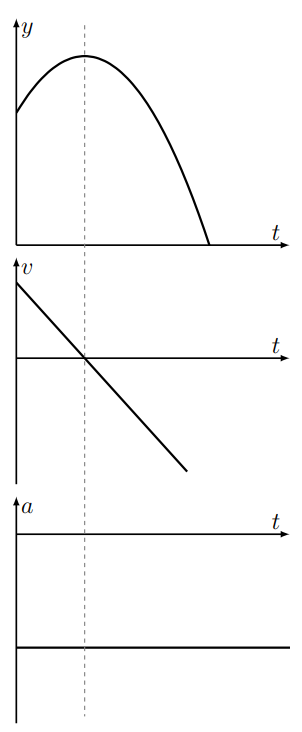
15. Answer Examples \(4.11\) and \(4.12\) when \(g=5 \mathrm{~m} / \mathrm{s}^{2}, v_{0}=20 \mathrm{~m} / \mathrm{s}\) and \(y_{0}=100 \mathrm{~m}\).
16. What is the dashed line in Figure 4.1 indicating?

Featured Problem \(4.3\) (How to outrun a cheetah): A cheetah can run at top speed \(v_{c}\) but it has to slow down (decelerate) to keep from getting too hot. Assume that the cheetah has a constant rate of (negative) acceleration \(a=-a_{c}\). A gazelle runs at a slower speed \(v_{g}\) but it can maintain that constant speed for a long time. If the gazelle is initially a distance \(d\) from the cheetah, and running away, when would it be caught? Is there a (large enough) distance d such that it never gets caught?

A cheetah chasing a gazelle. Who will win the race?