4.3: Sketching the First and Second Derivative and the Anti-Derivatives
- Page ID
- 121104

\( \newcommand{\vecs}[1]{\overset { \scriptstyle \rightharpoonup} {\mathbf{#1}} } \)
\( \newcommand{\vecd}[1]{\overset{-\!-\!\rightharpoonup}{\vphantom{a}\smash {#1}}} \)
\( \newcommand{\id}{\mathrm{id}}\) \( \newcommand{\Span}{\mathrm{span}}\)
( \newcommand{\kernel}{\mathrm{null}\,}\) \( \newcommand{\range}{\mathrm{range}\,}\)
\( \newcommand{\RealPart}{\mathrm{Re}}\) \( \newcommand{\ImaginaryPart}{\mathrm{Im}}\)
\( \newcommand{\Argument}{\mathrm{Arg}}\) \( \newcommand{\norm}[1]{\| #1 \|}\)
\( \newcommand{\inner}[2]{\langle #1, #2 \rangle}\)
\( \newcommand{\Span}{\mathrm{span}}\)
\( \newcommand{\id}{\mathrm{id}}\)
\( \newcommand{\Span}{\mathrm{span}}\)
\( \newcommand{\kernel}{\mathrm{null}\,}\)
\( \newcommand{\range}{\mathrm{range}\,}\)
\( \newcommand{\RealPart}{\mathrm{Re}}\)
\( \newcommand{\ImaginaryPart}{\mathrm{Im}}\)
\( \newcommand{\Argument}{\mathrm{Arg}}\)
\( \newcommand{\norm}[1]{\| #1 \|}\)
\( \newcommand{\inner}[2]{\langle #1, #2 \rangle}\)
\( \newcommand{\Span}{\mathrm{span}}\) \( \newcommand{\AA}{\unicode[.8,0]{x212B}}\)
\( \newcommand{\vectorA}[1]{\vec{#1}} % arrow\)
\( \newcommand{\vectorAt}[1]{\vec{\text{#1}}} % arrow\)
\( \newcommand{\vectorB}[1]{\overset { \scriptstyle \rightharpoonup} {\mathbf{#1}} } \)
\( \newcommand{\vectorC}[1]{\textbf{#1}} \)
\( \newcommand{\vectorD}[1]{\overrightarrow{#1}} \)
\( \newcommand{\vectorDt}[1]{\overrightarrow{\text{#1}}} \)
\( \newcommand{\vectE}[1]{\overset{-\!-\!\rightharpoonup}{\vphantom{a}\smash{\mathbf {#1}}}} \)
\( \newcommand{\vecs}[1]{\overset { \scriptstyle \rightharpoonup} {\mathbf{#1}} } \)
\( \newcommand{\vecd}[1]{\overset{-\!-\!\rightharpoonup}{\vphantom{a}\smash {#1}}} \)
- Given a sketch of a function, sketch its first and second derivatives.
- Given the sketch of a function, sketch its first and second antiderivatives.
We continue to practice sketching derivatives (first and second) as well as antiderivatives, given a sketch of the original function. Here, we aim for qualitative features, where only the most important aspects of the graphs (locations of key points such as peaks and troughs) are indicated.
Sketch the first and second derivatives of the functions in Figure 4.2.

Solution
In Figure \(4.3\) we show the functions \(y(t)\) (top row), their first derivatives \(y^{\prime}(t)\) (middle row), and the second derivatives \(y^{\prime \prime}(t)\) (bottom row). In each case, we determined the slopes of tangent lines as a first step.

Along flat parts of the graph), the derivative is zero. This is indicated at several places in Figure 4.3. In (b), there are cusps at which derivatives are not defined.
- Identify any cusps in Figure 4.2.
- What is each dotted line indicating in Figure 4.3?
- What is the arrow in the middle of Figure \(4.3\) indicating?
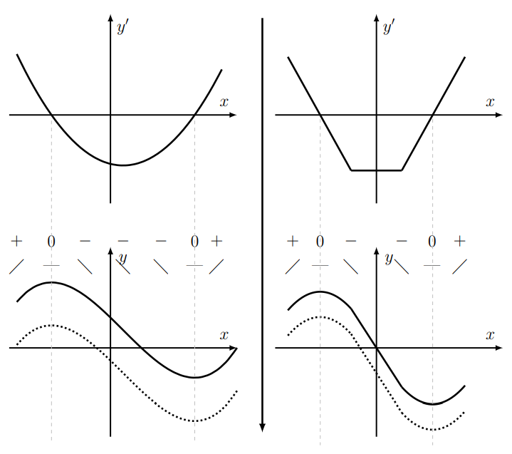
Sketch the antiderivatives \(y(x)\) for each derivative \(y^{\prime}(x)\) shown in Figure 4.4.

Solution
An antiderivative is only defined up to some (additive) constant. In the bottom panels of Figure \(4.5\) we show sample antiderivatives for each case. If we are given additional information, for example that \(y(0)=0\), we could then select one specific curve out of this family of solutions. A second point to observe is that antidifferentiation smoothes a function. Even though \(y^{\prime}(x)\) has cusps in (b), we find that \(y(x)\) is smooth. We later see that the points at which \(y^{\prime}(x)\) has a cusp correspond to places where the concavity of \(y(x)\) changes abruptly.