
6.4: Summary
- Page ID
- 121115

\( \newcommand{\vecs}[1]{\overset { \scriptstyle \rightharpoonup} {\mathbf{#1}} } \)
\( \newcommand{\vecd}[1]{\overset{-\!-\!\rightharpoonup}{\vphantom{a}\smash {#1}}} \)
\( \newcommand{\id}{\mathrm{id}}\) \( \newcommand{\Span}{\mathrm{span}}\)
( \newcommand{\kernel}{\mathrm{null}\,}\) \( \newcommand{\range}{\mathrm{range}\,}\)
\( \newcommand{\RealPart}{\mathrm{Re}}\) \( \newcommand{\ImaginaryPart}{\mathrm{Im}}\)
\( \newcommand{\Argument}{\mathrm{Arg}}\) \( \newcommand{\norm}[1]{\| #1 \|}\)
\( \newcommand{\inner}[2]{\langle #1, #2 \rangle}\)
\( \newcommand{\Span}{\mathrm{span}}\)
\( \newcommand{\id}{\mathrm{id}}\)
\( \newcommand{\Span}{\mathrm{span}}\)
\( \newcommand{\kernel}{\mathrm{null}\,}\)
\( \newcommand{\range}{\mathrm{range}\,}\)
\( \newcommand{\RealPart}{\mathrm{Re}}\)
\( \newcommand{\ImaginaryPart}{\mathrm{Im}}\)
\( \newcommand{\Argument}{\mathrm{Arg}}\)
\( \newcommand{\norm}[1]{\| #1 \|}\)
\( \newcommand{\inner}[2]{\langle #1, #2 \rangle}\)
\( \newcommand{\Span}{\mathrm{span}}\) \( \newcommand{\AA}{\unicode[.8,0]{x212B}}\)
\( \newcommand{\vectorA}[1]{\vec{#1}} % arrow\)
\( \newcommand{\vectorAt}[1]{\vec{\text{#1}}} % arrow\)
\( \newcommand{\vectorB}[1]{\overset { \scriptstyle \rightharpoonup} {\mathbf{#1}} } \)
\( \newcommand{\vectorC}[1]{\textbf{#1}} \)
\( \newcommand{\vectorD}[1]{\overrightarrow{#1}} \)
\( \newcommand{\vectorDt}[1]{\overrightarrow{\text{#1}}} \)
\( \newcommand{\vectE}[1]{\overset{-\!-\!\rightharpoonup}{\vphantom{a}\smash{\mathbf {#1}}}} \)
\( \newcommand{\vecs}[1]{\overset { \scriptstyle \rightharpoonup} {\mathbf{#1}} } \)
\( \newcommand{\vecd}[1]{\overset{-\!-\!\rightharpoonup}{\vphantom{a}\smash {#1}}} \)
- We can improve the accuracy of a sketch of a function \(f(x)\) by examining its derivatives. For example, if \(f^{\prime}(x)>0\) then \(f(x)\) is increasing, and if \(f^{\prime}(x)<0\), then \(f(x)\) is decreasing. Further, if \(f^{\prime \prime}(x)>0\) then this corresponds to \(f^{\prime}(x)\) increasing, which means \(f(x)\) is concave up. Similarly, \(f^{\prime \prime}(x)<0\) corresponds to \(f(x)\) being concave down.
- If \(f^{\prime \prime}\left(x_{0}\right)=0\) and \(f^{\prime \prime}(x)\) changes sign at \(x_{0}\), then \(x_{0}\) is a point of inflection of \(f(x)\) : a point where its concavity changes.
- If \(f^{\prime}\left(x_{0}\right)=0\), then \(x_{0}\) is a critical point of the function \(f(x)\). A critical point needs to be further tested to determine whether it is a local minimum, local maximum or neither.
- Given a critical point \(x_{0}\) (where \(f^{\prime}\left(x_{0}\right)=0\) ), the first derivative test examines the sign of \(f^{\prime}(x)\) near \(x_{0}\). If the sign pattern of \(f^{\prime}(x)\) is \(+, 0,-\) (from left to right as we cross \(x_{0}\) ), then \(x_{0}\) is a local maximum. If the sign pattern is \(-, 0,+\), then \(x_{0}\) is a local minimum.
- Given a critical point \(x_{0}\) (where \(f^{\prime}\left(x_{0}\right)=0\) ), the second derivative test examines the sign of \(f^{\prime \prime}\left(x_{0}\right)\). If \(f^{\prime \prime}\left(x_{0}\right)<0\), then \(x_{0}\) is a local maximum. If \(f^{\prime \prime}\left(x_{0}\right)>0\), then \(x_{0}\) is a local minimum. If \(f^{\prime \prime}\left(x_{0}\right)=0\), the second derivative test is inconclusive.
- A global maximum and minimum can only be identified after comparing the values of the function at all critical points and endpoints of the interval. (Remark: For discontinuous or non-smooth functions, we must also examine values of \(f\) at points of discontinuity and cusps, not discussed in this chapter).
- Consider the function depicted below:
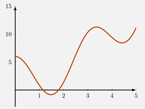
- Circle all zeros.
- Where are the local maxima?
- How many local minima are there?
- Where does the function change sign?
- Draw a graph to justify that if \(f^{\prime}(x)>0\), then \(f(x)\) is increasing.
- Where does the function \(f(a)=a^{3}(a-\pi)(a+\rho)^{5}(a-2)^{2}\) change signs?
- Suppose you are given that \(\gamma\) is a critical point of some function \(g\). What would you ask to learn more about the shape of \(g\) ?