6.3: Sketching the Graph of a Function

Learning Objectives

1. Given a function (polynomial, rational, etc.) be able to find its zeros, critical points, inflection points, and determine where it is increasing or decreasing, concave up or down.
2. Using a combination of the above techniques, together with methods of Section 1.4, assemble a reasonably accurate sketch of the graph of a function.
3. Using these techniques, identify all local as well as global extrema (minima and maxima) of a function \(f(x)\) on an interval \(a \leq x \leq b\).

In Section 1.4, we used elementary reasoning about power functions to sketch the graph of simple polynomials. Now that we have learned more advanced calculus techniques, we can hone such methods to produce more accurate sketches of the graph of a function. We devote this section to illustrating some examples.

Example 6.8

Sketch the graph of the function \(B(x)=C\left(x^{2}-x^{3}\right)\). Assume that \(C>0\) is constant.

Solution

To prepare, we compute the derivatives:

\[B^{\prime}(x)=C\left(2 x-3 x^{2}\right), \quad B^{\prime \prime}(x)=C(2-6 x) . \nonumber \]

1. Zeros. We start by finding the zeros of the function. Factoring makes this easy. Solving \(B(x)=0\), we find

\[0=C\left(x^{2}-x^{3}\right)=C x^{2}(1-x), \quad \Rightarrow \quad \Rightarrow \quad x=0,1 . \nonumber \]

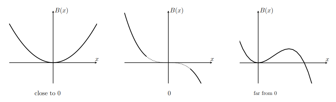
2. Consider the powers. Reasoning about the powers as in Chapter 1 , we surmise that close to the origin, \(x^{2}\) dominates (producing a parabolic shape) whereas, far away, \(-x^{3}\) dominates (producing the shape of an inverted cubic). We show this in a preliminary sketch, Figure 6.6.

Figure 6.6: Figure for the function \(B(x)=\) \(C\left(x^{2}-x^{3}\right)\) in Example \(6.8\) showing which power dominates.

3. First derivative. To find critical points, set \(B^{\prime}(x)=0\), obtaining

\[\begin{array}{rlr} B^{\prime}(x)=C\left(2 x-3 x^{2}\right)=0, & \Rightarrow & 0=2 x-3 x^{2}=x(2-3 x), \\ & \Rightarrow & x=0, \frac{2}{3} \end{array} \nonumber \]

By considering the sketch in Figure 6.6, we can see that \(x=0\) is a local minimum, and \(x=2 / 3\) a local maximum. Confirmation of this comes from the second derivative.

4. Second derivative. From the second derivative, \(B^{\prime \prime}(0)=2>0\), confirming that \(x=0\) is a local minimum. Further, \(B^{\prime \prime}(2 / 3)=2-6 \cdot(2 / 3)=-2<0\) so \(x=2 / 3\) is a local maximum, as expected.
5. Classifying the critical points. Now identifying where \(B^{\prime \prime}(x)=0\), we find that

\[B^{\prime \prime}(x)=C(2-6 x)=0, \quad \text { when } \quad 2-6 x=0 \quad \Rightarrow \quad x=\frac{2}{6}=\frac{1}{3} \nonumber \]

we also note that the second derivative changes sign here: i.e. for \(x<1 / 3\), \(B^{\prime \prime}(x)>0\) and for \(x>1 / 3, B^{\prime \prime}(x)<0\). We may conclude that there is an inflection point at \(x=1 / 3\). The final sketch, now labeled, is given in Figure 6.7.

Figure 6.7: A sketch of \(B(x)=C\left(x^{2}-x^{3}\right)\) in Example \(6.8\).

Steps in the calculations of Example \(6.8\).

Mastered Material Check

8. What is the independent variable in Example 6.8? The dependent variable?
9. Given our discussion on "considering the powers" for Example 6.8, add a reasonable scale to each of \(x\)-axes for the graphs in Figure 6.6.

Example 6.9

Sketch the graph of the function \(y=f(x)=8 x^{5}+5 x^{4}-20 x^{3}\)

Solution

This example is more challenging, but similar ideas apply.

1. Zeros. Factoring the expression for \(y\) and then using the quadratic formula leads to

\[y=x^{3}\left(8 x^{2}+5 x-20\right) . \quad \Rightarrow \quad x=0,-\frac{5}{16} \pm \frac{1}{16} \sqrt{665} . \nonumber \]

In decimal form, these are approximately \(x=0,1.3,-1.92\).

2. Consider the powers. The highest power is \(8 x^{5}\), so far from the origin we expect typical positive odd function behavior. The lowest power is \(-20 x^{3}\), which means that close to zero, we expect to see a negative cubic. This implies that the function "turns around", creating local maxima and minima. We draw a rough sketch in Figure \(6.8\).

Figure 6.8: \(y=f(x)=8 x^{5}+5 x^{4}-20 x^{3}\). From Example 6.9, this function behaves roughly like the negative cubic near the origin, and like \(8 x^{5}\) for large \(x\).

3. First derivative. Calculating the derivative of \(f(x)\) and then factoring leads to

\[\frac{d y}{d x}=f^{\prime}(x)=40 x^{4}+20 x^{3}-60 x^{2}=20 x^{2}(2 x+3)(x-1) \nonumber \]

so this derivative is zero at: \(x=0,1,-3 / 2\). We expect critical points at these places.

4. Second derivative. We calculate the second derivative and factor to obtain

\[\frac{d^{2} y}{d x^{2}}=f^{\prime \prime}(x)=160 x^{3}+60 x^{2}-120 x=20 x\left(8 x^{2}+3 x-6\right) . \nonumber \]

Thus, the second derivative is zero at

\[x=0,-\frac{3}{16}+\frac{1}{16} \sqrt{201},-\frac{3}{16}-\frac{1}{16} \sqrt{201} . \nonumber \]

The values of these roots can be approximated by: \(x=0,0.69,-1.07\).

5. Classifying the critical points. To identify the types of critical points, we use the second derivative test.

• \(f^{\prime \prime}(0)=0\) so the test is inconclusive at \(x=0\).
• \(f^{\prime \prime}(1)=20(8+3-6)>0\) implies a local minimum \(x=1\), and
• \(f^{\prime \prime}(-3 / 2)=-225<0\) implies a local maximum at \(x=-3 / 2\).

We summarize the results in Table 6.1.

Table 6.1: \(y=x^{3}\left(8 x^{2}+5 x^{2}-20\right)\) and its detailed behavior.

\(\boldsymbol{x}=\)	\(-1.92\)	\(-1.5\)	\(-1.07\)	0	\(0.69\)	1	\(1.3\)
\(\boldsymbol{f}(\boldsymbol{x})=\)	0	\(32.0\)		0		\(-7\)	0
\(\boldsymbol{f}^{\prime}(\boldsymbol{x})=\)		0		0		0
\(\boldsymbol{f}^{\prime \prime}(\boldsymbol{x})=\)		\(<0\)	0	0	0	\(>0\)
characteristic:	zero	max	inflection	inflection	min	zero

The shape of the function, its first and second derivatives are shown in Figure 6.9.

Figure 6.9: The function \(y=f(x)=\) \(8 x^{5}+5 x^{4}-20 x^{3}\), and its first and second derivatives, \(f^{\prime}(x)\) and \(f^{\prime \prime}(x)\).

Mastered Material Check

11. Use software to verify the plot of the function \(y=f(x)\) in Example 6.9. Then plot \(2 y\). What changes?

Global maxima and minima, endpoints of an interval

A global maximum (also denoted absolute maximum) of a function over some interval is the largest value that the function attains on that interval. Similarly a global minimum (or absolute minimum) is the smallest value.

Note. For a function defined on a closed interval, we must check critical points and endpoints of the interval to determine where global maxima and minima occur, as illustrated in Example 6.10.

Example 6.10

Consider \(y=f(x)=\frac{2}{x}+x^{2}\) on the interval \(0.1 \leq x \leq 4\). Find the absolute maximum and minimum.

Solution

We first compute the derivatives:

\[f^{\prime}(x)=-2 \frac{1}{x^{2}}+2 x, \quad f^{\prime \prime}(x)=4 \frac{1}{x^{3}}+2 . \nonumber \]

Solving for critical points by setting \(f^{\prime}(x)=0\), we find

\[-2 \frac{1}{x^{2}}+2 x=0, \quad \Rightarrow \quad-2 \frac{1}{x^{2}}=2 x \quad \Rightarrow \quad x^{3}=1 \nonumber \]

which implies a critical point at \(x=1\). The second derivative at this point is

\[f^{\prime \prime}(1)=4 \frac{1}{1^{3}}+2=6>0, \nonumber \]

so that \(x=1\) is a local minimum.

Figure 6.10: The function \(f(x)=\frac{2}{x}+x^{2}\) on the interval \(0.1<x<4\) has no local maximum.

We now calculate the value of the function at the endpoints \(x=0.1\) and \(x=4\) and at the critical point \(x=1\) to determine where global and local minima and/or maxima occur:

• \(f(0.1)=\frac{2}{0.1}+0.1^{2}=20.01\);
• \(f(1)=\frac{2}{1}+1^{2}=3\);
• \(f(4)=\frac{2}{4}+4^{2}=16.5\).

Consequently, \(x=1\) is both a local minimum and the global minimum on the given interval. There are no local maxima. The global maximum occurs at the left endpoint, \(x=0\).1. Figure \(6.10\) confirms our conclusions.

Steps in Example 6.10: Finding the absolute minimum and maximum of a function on a given interval.