6.2: Special Points on the Graph of a Function

Learning Objectives

1. Define a zero of a function and be able to identify zeros for simple functions (factorizable polynomials).
2. Explain that a function \(f(x)\) can have various types of critical points (maxima, minima, and other types) at which \(f^{\prime}(x)=0\).
3. Find critical points for a given function.
4. Using first or second derivative tests, classify a given critical point as a maximum, minimum (or neither).

In this section we use tools of algebra and calculus to identify special points on the graph of a function. We first consider the zeros of a function, and then its critical points.

Zeros of a function

Example 6.4 (Factoring)

For the function \(y=f(x)=x^{2}-5 x+6\), find zeros by factoring.

Solution

This polynomial has factors \(f(x)=(x-3)(x-2)\). Zeros are values of \(x\) satisfying \(0=(x-3)(x-2)\), so either \((x-3)=0\) or \((x-2)=0\). Hence, there are two zeros, \(x=2,3\).

Example 6.5

Find the zeros of the function \(y=f(x)=x^{3}-3 x^{2}+x\).

Solution

We can factor this function into \(f(x)=x\left(x^{2}-3 x+1\right)\). From this we see that \(x=0\) is one of the desired zeros of \(f\). To find the others, we apply the quadratic formula to the second factor, obtaining

\[x_{1,2}=\frac{1}{2}\left(3 \pm \sqrt{3^{2}-4}\right)=\frac{1}{2}(3 \pm \sqrt{5}) . \nonumber \]

Thus, there are a total of three zeros in this case:

\[x=0, \quad \frac{1}{2}(3+\sqrt{5}), \quad \frac{1}{2}(3-\sqrt{5}) . \nonumber \]

Mastered Material Check

5. What is another term used for zeros of a function?

Example 6.6

Find zeros of the function \(y=f(x)=x^{3}-x-3\).

Solution

This polynomial does not factor into integers, nor is it easy to apply a cubic formula (analogous to the quadratic formula). However, as we saw in Example 5.10, Newton’s method leads to an accurate approximation for the only zero of this function, \((x \approx 1.6717)\)

Critical points

Clearly, a critical point occurs whenever the slope of the tangent line to the graph of the function is zero, i.e. the tangent line is horizontal. Figure \(6.4\) shows several possible shapes of the graph of a function close to a critical point. From left to right, these are a local maximum, a local minimum and two inflection points.

Definition 6.2

A critical point of the function \(f(x)\) is any point \(x\) at which the first derivative is zero, i.e. \(f^{\prime}(x)=0\).

Figure 6.4: A critical point (place where \(\left.f^{\prime}(x)=0\right)\) can be a local maximum, local minimum, or neither.

Critical points play an important role in many scientific applications, as described in Chapter 7. Hence, we seek criteria to determine whether a critical point is a local maximum, minimum, or neither.

Example 6.7

Consider the function \(y=f(x)=x^{3}+3 x^{2}+a x+1\). For what range of values of a are there no critical points for this function?

Solution

We compute the first derivative \(f^{\prime}(x)=3 x^{2}+6 x+a\). A critical point would occur whenever \(0=f^{\prime}(x)\), which implies \(0=3 x^{2}+6 x+a\). This is a quadratic equation whose solutions are

\[x_{1,2}=\frac{-6 \pm \sqrt{36-4 a \cdot 3}}{6} . \nonumber \]

There two real solutions provided the discriminant is positive, \(36-12 a>0\). However, when \(36-12 a<0\) (which corresponds to \(a>3\) ), there are no real solutions and consequently no critical points.

What happens close to a critical point

In Figure \(6.5\) we contrast the behavior of two functions (top row), each with a different type of critical point. We compare their first and second derivatives close to that point (second and third rows, respectively). In each case, the first derivative \(f^{\prime}(x)=0\) at the critical point.

Near the local maximum (moving from left to right), the slope of \(f(x)\) transitions from positive to zero (at the critical point) to negative. This means that \(f^{\prime}(x)\) is a decreasing function, as indicated in Figure 6.5. Since changes in the first derivative are measured by its derivative \(f^{\prime \prime}(x)\), we find that the second derivative is negative at a local maximum. The converse is true near a local minimum (right column in Figure 6.5).

Figure 6.5: Close to a local maximum, \(f(x)\) is concave down, \(f^{\prime}(x)\) is decreasing, so that \(f^{\prime \prime}(x)\) is negative. Close to a local minimum, \(f(x)\) is concave up, \(f^{\prime}(x)\) is increasing, so that \(f^{\prime \prime}(x)\) is positive.

A summary of types of critical points and how to tell them apart.

Mastered Material Check

6. Why are there no critical points when \(36-12 a<0\) for the function \(f(x ?)=x^{3}+3 x^{2}+a x+1\)

We collect and summarize conclusions about derivatives below.

Summary: first derivative

\(f^{\prime}(x)<0\)	\(f^{\prime}\left(x_{0}\right)=0\)	\(f^{\prime}(x)>0\)
decreasing function	critical point	increasing function
	at \(x_{0}\)

• The first derivative test: depends on changes in the sign of the first derivative close to a critical point, \(x_{0}\).

Near a local maximum, the sign pattern is:

1. \(x<x_{0}, f^{\prime}(x)>0\);
2. \(x=x_{0}, f^{\prime}\left(x_{0}\right)=0\);
3. \(x>x_{0}, f^{\prime}\left(x_{0}\right)<0\).

Near a local minimum, the sign pattern is:

1. \(x<x_{0}, f^{\prime}(x)<0\);
2. \(x=x_{0}, f^{\prime}\left(x_{0}\right)=0\);
3. \(x>x_{0}, f^{\prime}(x)>0\).

Summary: second derivative

\(f^{\prime \prime}(x)<0\)	\(f^{\prime \prime}\left(x_{0}\right)=0\)	\(f^{\prime \prime}(x)>0\)
curve concave down	inflection point	curve concave up
	at \(x_{0}\) only if \(f^{\prime \prime}\) changes sign

• The second derivative test: is based on the sign of \(f^{\prime \prime}\left(x_{0}\right)\) for \(x_{0}\) a critical point (satisfying \(f^{\prime}\left(x_{0}\right)=0\) ).

If \(f^{\prime \prime}\left(x_{0}\right)<0, x_{0}\) is a local maximum.

If \(f^{\prime \prime}\left(x_{0}\right)=0\), test is inconclusive about max/min at \(x_{0}\). If \(f^{\prime \prime}\) also changes sign at \(x_{0}\), then \(x_{0}\) is an inflection point.

If \(f^{\prime \prime}\left(x_{0}\right)>0, x_{0}\) is a local minimum.

Mastered Material Check

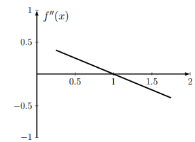
7. Given the following graph of a function’s second derivative, can you say anything about the concavity of the original function?