7.1: Simple Biological Optimization Problems

Learning Objectives

1. Given a function, find the derivative of that function and identify all critical points.
2. Using a combination of sketching and tests for critical points developed in Section \(6.2\), diagnose the type of critical point.

In the first examples, the function to optimize is specified, making the problem simply one of carefully applying calculus methods.

Mastered Material Check

How do you find the critical points of a function \(f(x)\)?

Density dependent (logistic) growth in a population

Biologists often notice that the growth rate of a population depends not only on the size of the population, but also on how crowded it is. Constant growth is not sustainable. When individuals have to compete for resources, nesting sites, mates, or food, they cannot invest time nor energy in reproduction, leading to a decline in the rate of growth of the population. Such population growth is called density dependent growth.

One common example of density dependent growth is called the logistic growth law. Here it is assumed that the growth rate of the population, \(G\) depends on the density of the population, \(N\), as follows:

\[G(N)=r N\left(\frac{K-N}{K}\right) . \nonumber \]

Here \(N\) is the independent variable, and \(G(N)\) is the function of interest. All other quantities are constant:

• \(r>0\) is a constant, called the intrinsic growth rate, and
• \(K>0\) is a constant, called the carrying capacity. It represents the population density that a given environment can sustain.

Importantly, when differentiating \(G\), we treat \(r\) and \(K\) as "numbers". A generic sketch of \(G\) as a function of \(N\) is shown in Figure 7.1.

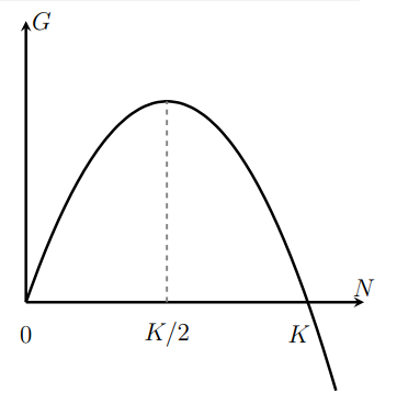
Figure 7.1: In logistic growth, the population growth rate rate \(G\) depends on population size \(N\) as shown here.

Mastered Material Check

2. Give an example of units for \(N\).
3. What units might \(G\) carry?

Example 7.1 (Logistic growth rate)

Answer the following questions:

1. Find the population density \(N\) that leads to the maximal growth rate \(G(N)\).
2. Find the value of the maximal growth in terms of \(r, K\).
3. For what population size is the growth rate zero?

Solution

We can expand \(G(N)\) :

\[G(N)=r N\left(\frac{K-N}{K}\right)=r N-\frac{r}{K} N^{2}, \nonumber \]

from which it is apparent that \(G(N)\) is a polynomial in powers of \(N\), with constant coefficients \(r\) and \(r / K\).

a) To find critical points of \(G(N)\), we find \(N\) such that \(G^{\prime}(N)=0\), and then test for maxima:

\[G^{\prime}(N)=r-2 \frac{r}{K} N=0 . \quad \Rightarrow \quad r=2 \frac{r}{K} N \quad \Rightarrow \quad N=\frac{K}{2} . \nonumber \]

Hence, \(N=K / 2\) is a critical point, but is it a maximum? We check this in one of several ways. First, a sketch in Figure \(7.1\) reveals a downwardsopening parabola. This confirms a local maximum. Alternately, we can apply a tool from Section \(6.2\) such as the second derivative test:

\[\begin{aligned} G^{\prime \prime}(N)=-2 \frac{r}{K}<0 & \Rightarrow \quad G(N) \text { concave down } \\ & \Rightarrow \quad N=\frac{K}{2} \text { is a local maximum } \end{aligned} \nonumber \]

Thus, the population density with the greatest growth rate is \(K / 2\).

b) The maximal growth rate is found by evaluating the function \(G\) at the critical point, \(N=K / 2\),

\[G\left(\frac{K}{2}\right)=r\left(\frac{K}{2}\right)\left(\frac{K-\frac{K}{2}}{K}\right)=r \frac{K}{2} \cdot \frac{1}{2}=\frac{r K}{4} . \nonumber \]

c) To find the population size at which the growth rate is zero, we set \(G=0\) and solve for \(N\) :

\[G(N)=r N\left(\frac{K-N}{K}\right)=0 . \nonumber \]

There are two solutions. One is trivial: \(N=0\). (This is biologically interesting in the sense that it rules out the ancient idea of spontaneous generation - a defunct theory that held that life can arise on its own, from dust or air. If \(N=0\), the growth rate is also 0 , so no population spontaneously arises according to logistic growth.) The second solution, \(N=K\) means that the population is at its "carrying capacity".

We return to this type of growth in Chapter 13.

Cell size for maximal nutrient accumulation rate

According to the model of Section 1.2, the nutrient absorption and consumption rates, \(A(r), C(r)\), of a simple spherical cell of radius \(r\) are:

\[A(r)=k_{1} S=4 k_{1} \pi r^{2}, \quad C(r)=k_{2} V=\frac{4}{3} \pi k_{2} r^{3}, \nonumber \]

for \(k_{1}, k_{2}>0\) constants. The net rate of increase of nutrients, which is the difference of the two is:

\[N(r)=A(r)-C(r)=4 k_{1} \pi r^{2}-\frac{4}{3} \pi k_{2} r^{3} \]

This quantity is a function of the radius \(r\) of the cell.

Example 7.2

Determine the radius of the cell for which the net rate of increase of nutrients \(N(r)\) is largest.

Solution

We are asked to maximize \(N(r)\) with respect to \(r\). We first find critical points of \(N(r)\), keeping in mind that \(8 k_{1} \pi\) and \(4 k_{2} \pi\) are constant for the purpose of differentiation. Critical points occur when \(N^{\prime}(r)=0\), i.e.

\[\begin{aligned} N^{\prime}(r)=8 k_{1} \pi r-4 k_{2} \pi r^{2}=0 & \Rightarrow \quad 4 \pi r\left(2 k_{1}-k_{2} r\right)=0 \\ & \Rightarrow \quad r=0, \quad 2 \frac{k_{1}}{k_{2}} \end{aligned} \nonumber \]

To identify the type of critical point, we use the second derivative test

\[N^{\prime \prime}(r)=8 k_{1} \pi-8 k_{2} \pi r=8 \pi\left(k_{1}-k_{2} r\right) . \nonumber \]

Substituting in \(r=2 k_{1} / k_{2}\), we find that

\[N^{\prime \prime}\left(2 \frac{k_{1}}{k_{2}}\right)=8 \pi\left(k_{1}-k_{2} \frac{2 k_{1}}{k_{2}}\right)=-8 \pi k_{1}<0 . \nonumber \]

Thus, the second derivative is negative at at \(r=2 k_{1} / k_{2}\), verifying that this is a local maximum. Hence the net rate of nutrient uptake is greatest for cells of radius \(r=2 k_{1} / k_{2}\)

Mastered Material Check

4. Give example units for each of \(A(r), C(r)\) and \(N(r)\). Are there restrictions in place?