9.3: The Power Rule for Fractional Powers

Implicit differentiation is a useful technique for finding derivatives of inverse functions. Here we use the known power rule for \(y=x^{2}\) to find the derivative of its inverse function, \(y=\sqrt{x}=x^{1 / 2}\). This general idea recurs in later chapters when we introduce new functions and their inverses.

Example 9.7: Derivative of \(\sqrt{x}\)

Consider the function \(y=\sqrt{x}=x^{1 / 2}\). Use implicit differentiation to compute the derivative of this function.

Solution

Let us rewrite the relationship \(y=\sqrt{x}\) in the form \(y^{2}=x\), but consider \(y\) as the dependent variable, i.e. when we differentiate, we remember that \(y\) depends on \(x\) :

\[[y(x)]^{2}=x . \nonumber \]

Taking derivatives of both sides leads to

\[\frac{d}{d x}\left([y(x)]^{2}\right)=\frac{d}{d x}(x) \Rightarrow 2[y(x)] \frac{d y}{d x}=1 \quad \Rightarrow \quad \frac{d y}{d x}=\frac{1}{2 y} . \nonumber \]

We eliminate \(y\) by substituting \(y=\sqrt{x}\). Then

\[\frac{d y}{d x}=\frac{1}{2 \sqrt{x}}=\frac{1}{2} x^{-1 / 2} . \nonumber \]

This verifies the power law for the above example.

A similar procedure can be applied to any power function with fractional power. When we apply similar steps, we get the following rule:

Derivative of fractional-power function:

The derivative of

\[y=f(x)=x^{m / n} \nonumber \]

is\[\frac{d y}{d x}=\frac{m}{n} x^{\left(\frac{m}{n}-1\right)} . \nonumber \]

Using implicit differentiation to compute the derivative of \(y=\sqrt{x}\).

Mastered Material Check

14. Justify the derivative of the fractional power rule by actually carrying out an implicit differentiation calculation.

Example 9.8 (The astroid)

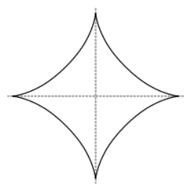
The curve

\[x^{2 / 3}+y^{2 / 3}=2^{2 / 3} \nonumber \]

has the shape of an astroid. It describes the shape (Figure 9.10) generated by a the path of a point on the perimeter of a disk of radius \(\frac{1}{2}\) rolling inside the perimeter of a circle of radius 2.

Find the slope of the tangent line to a point on the astroid.

Figure 9.10: The astroid is generated by a disk or radius \(1 / 2\) rolling inside a circle of radius 2.

Solution

Considering \(y\) as the dependent variable, we use implicit differentiation as follows:

\[\begin{aligned} \frac{d}{d x}\left(x^{2 / 3}+[y(x)]^{2 / 3}\right)=\frac{d}{d x} 2^{2 / 3} & \Rightarrow \quad \frac{2}{3} x^{-1 / 3}+\frac{d}{d y}\left(y^{2 / 3}\right) \frac{d y}{d x}=0 \\ & \Rightarrow \quad \frac{2}{3} x^{-1 / 3}+\frac{2}{3} y^{-1 / 3} \frac{d y}{d x}=0 \\ & \Rightarrow \quad x^{-1 / 3}+y^{-1 / 3} \frac{d y}{d x}=0 \\ & \Rightarrow \quad \frac{d y}{d x}=-\frac{x^{-1 / 3}}{y^{-1 / 3}} \end{aligned} \nonumber \]

The derivative fails to exist at \(x=0\) (where \(x^{-1 / 3}\) is undefined) and at \(y=0\) (where \(y^{-1 / 3}\) is undefined).

See Demo created by David Austin of the astroid.

Mastered Material Check

15. Point out places on Figure \(9.10\) at which the derivative fails to exist, and explain the properties of those specific points on the astroid.

Example 9.9 (Horizontal tangent and concavity on a rotated ellipse)

Find the highest point on the (rotated) ellipse \(x^{2}+3 y^{2}-x y=1\).

Solution

1. Finding the slope of the tangent line: By implicit differentiation,

\[\frac{d}{d x}\left[x^{2}+3 y^{2}-x y\right]=\frac{d}{d x} 1 \Rightarrow \frac{d\left(x^{2}\right)}{d x}+\frac{d\left(3 y^{2}\right)}{d x}-\frac{d(x y)}{d x}=0 \nonumber \]

We must use the product rule to compute the derivative of the last term \(x y\) :

\[2 x+6 y \frac{d y}{d x}-\left(x \frac{d y}{d x}+\frac{d x}{d x} y\right)=0 \quad \Rightarrow \quad 2 x+6 y \frac{d y}{d x}-x \frac{d y}{d x}-1 y=0 . \nonumber \]

Grouping terms, we have

\[(6 y-x) \frac{d y}{d x}+(2 x-y)=0 \quad \Rightarrow \quad \frac{d y}{d x}=\frac{(y-2 x)}{(6 y-x)} . \nonumber \]

Setting \(d y / d x=0\), we obtain \(y-2 x=0\) so that \(y=2 x\) at the point of interest. Next, we find the coordinates of the point.

2. Determining the coordinates of the point we want: We look for a point that satisfies the equation of the curve as well as the condition \(y=2 x\). There
   Using implicit differentiation to find the points on the top and bottom of the ellipse in Example 9.9. are two equations and two unknowns. Plugging \(y=2 x\) into the original equation of the ellipse, we get:

\[x^{2}+3 y^{2}-x y=1 \quad \Rightarrow \quad x^{2}+3(2 x)^{2}-x(2 x)=1 . \nonumber \]

After simplifying, this equation becomes \(11 x^{2}=1\), leading to the two possibilities

\[x=\pm \frac{1}{\sqrt{11}}, \quad y=\pm \frac{2}{\sqrt{11}} . \nonumber \]

Which of these two points is at the top? The rotated ellipse is depicted in Figure \(9.11\) which gives strong indication it is the positive solution - but we can confirm this analytically.

3. Identifying the point at the top: The top point on the ellipse is located at a point where the curve is concave down. Concavity can be determined using the second derivative, computed (from the first derivative) using the quotient rule:

\[\begin{aligned} y^{\prime \prime} & =\frac{[y-2 x]^{\prime}(6 y-x)-[6 y-x]^{\prime}(y-2 x)}{(6 y-x)^{2}} \\ & =\frac{\left[y^{\prime}-2\right](6 y-x)-\left[6 y^{\prime}-1\right](y-2 x)}{(6 y-x)^{2}} . \end{aligned} \nonumber \]

4. Plugging in information about the point: Now that we have set down the form of this derivative, we make some important observations about the specific point of interest. (This is done as a final step, only after all derivatives have been calculated)

• We are only concerned with the sign of the second derivative. The denominator is always positive (since it is squared) and so does not affect the sign.
• At the top of ellipse, \(y^{\prime}=0\), simplifying some of the terms above.
• At the top of ellipse, \(y=2 x\) so the term \((y-2 x)=0\).

We can thus simplify the expression for the \(y^{\prime \prime}\) to obtain

\[y^{\prime \prime}(x)=\frac{[-2](6 y-x)-[-x](0)}{(6 y-x)^{2}}=\frac{[-2](6 y-x)}{(6 y-x)^{2}}=\frac{-2}{(6 y-x)} . \nonumber \]

Using the fact that \(y=2 x\), we get the final form

\[y^{\prime \prime}(x)=\frac{-2}{(6(2 x)-x)}=\frac{-2}{11 x} . \nonumber \]

Consequently, the second derivative is negative (implying concave down curve) whenever \(x\) is positive. This tells us that at the point with positive \(x\) value \((x=1 / \sqrt{11})\), we are at the top of the ellipse. A graph of this curve is shown in Figure 9.11.

Figure 9.11: A rotated ellipse. In Example 9.9, we find the point at the top of the ellipse using implicit differentiation.

Mastered Material Check

16. Verify by hand that \(x=\pm \frac{1}{\sqrt{11}}\) are two possible solutions to Example 9.9.
17. Repeat Example \(9.9\) looking for the lowest point on the rotated ellipse.

Featured Problem 9.3 (Tangent to an ellipse): Find the equation of a line through the origin that is tangent to the ellipse

\[(x-a)^{2}+\frac{y^{2}}{s^{2}}=1 . \nonumber \]

This ellipse has its center at \((a, 0)\) and has axes 1 and \(s\).