9.2: Implicit Differentiation

Learning Objectives

1. Identify the distinction between a function that is defined explicitly and one that is defined implicitly.
2. Describe implicit differentiation geometrically.
3. Compute the slope of a curve at a given point using implicit differentiation, find tangent line equations, and solve problems based on such ideas.

Implicit and explicit definition of a function

A review of the definition of a function (e.g. Appendix C) reminds us that for a given \(x\) value, only one \(y\) value is permitted. For example, for

\[y=x^{2} \nonumber \]

any value of \(x\) leads to a single \(y\) value (Figure 9.7a).

Figure 9.7: (a) A function has to satisfy the vertical line property. Hence, the curve shown in (b) cannot be a function. We can write down an equation for the curve, but we cannot solve for \(y\) explicitly. (c) However, close to a given point on the curve (dark point), we can think of how changing the \(x\) coordinate of the point (shaded interval on \(x\) axis) leads to a change in the corresponding \(y\) coordinate on the same curve (shaded interval on \(y\) axis). (d) We can also ask what is the slope of the curve at the given point. This corresponds to \(\lim _{\Delta x \rightarrow 0} \Delta y / \Delta x\). Implicit differentiation can be used to compute that derivative.

Geometrically, this means that the graph of this function satisfies the vertical line property: a given \(x\) value can have at most one corresponding \(y\) value. Not all curves satisfy this property. The elliptical curve in Figure \(9.7 \mathrm{~b}\) clearly fails this, intersecting some vertical lines twice. This simply means that, while we can write down an equation for such a curve, e.g.

\[\frac{(x-1)^{2}}{4}+(y-1)^{2}=1, \nonumber \]

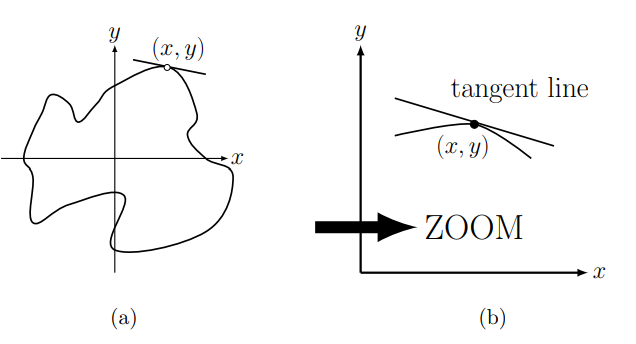
we cannot solve for a simple function that describes the entire curve. Nevertheless, the idea of a tangent line to such a curve - and consequently the slope of such a tangent line - is perfectly reasonable.

In order to make sense of this idea, we restrict attention to a local part of the curve, close to some point of interest (Figure 9.7c). Then near this point, the equation of the curve defines an implicit function, that is, close enough to the point of interest, a value of \(x\) leads to a unique value of \(y\). We refer to this value as \(y(x)\) to remind us of the relationship between the two variables.

How can we generalize the notion of a derivative to implicit functions? We observe from (Figure 9.7d) that a small change in \(x\) leads to a small change in \(y\). Without writing down an explicit expression for \(y\) versus \(x\), we can still determine these small changes, and form a ratio \(\Delta y / \Delta x\) which is a (secant line) slope. Now let \(\Delta x \rightarrow 0\) to arrive at the slope of a tangent line as before, \(d y / d x\). In the next section we show how to do this using implicit differentiation, an application of the chain rule.

Slope of a tangent line at the point on a curve

We now compute the tangent line at a point in several examples where it is inconvenient or impossible, to isolate \(y\) as a function of \(x\) (see Figure 9.8).

Figure 9.8: The curve in (a) is not a function and hence it can only be described implicitly. However, if we zoom in to a point in (b), we can define the derivative as the slope of the tangent line to the curve at the point of interest.

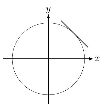
First, consider the simple example of a circle. We aim to find the slope of the tangent line at some point. The equation of a circle of radius 1 and centre at the origin \((0,0)\) is

\[x^{2}+y^{2}=1 . \nonumber \]

Here, the two variables are linked in a symmetric relationship. We can solve for \(y\), obtaining not one but two functions.

\[\begin{array}{rc} \text { top of circle: } & y=f_{1}(x)=\sqrt{1-x^{2}}, \\ \text { and bottom of circle: } & y=f_{2}(x)=-\sqrt{1-x^{2}} . \end{array} \nonumber \]

However, this makes the work of differentiation more complicated than necessary. Instead, we use implicit differentiation.

A brief introduction to implicit differentiation and slope of a tangent line to a circle.

Example 9.5 (Tangent to a circle)

1. Use implicit differentiation to find the slope of the tangent line to the point \(x=1 / 2\) in the first quadrant on a circle of radius 1 and centre at \((0,0)\).
2. Find the second derivative \(d^{2} y / d x^{2}\) at the same point.

Figure 9.9: Tangent line to a circle by implicit differentiation.

Solution

a) When \(x=1 / 2\) then \(y=\pm \sqrt{1-(1 / 2)^{2}}=\pm \sqrt{3} / 2\). The point in the first quadrant has \(y\) coordinate \(y=+\sqrt{3} / 2\).

Viewing \(x\) as the independent variable locally, (and \(y\) depending on \(x\) on the curve) we write

\[x^{2}+[y(x)]^{2}=1 \nonumber \]

Differentiating each side with respect to \(x\) :

\[\frac{d}{d x}\left(x^{2}+[y(x)]^{2}\right)=\frac{d}{d x} 1=0 \quad \Rightarrow \quad\left(\frac{d x^{2}}{d x}+\frac{d}{d x}[y(x)]^{2}\right)=0 \nonumber \]

Notice that in the second term, the value of \(x\) determines \(y\) which in turn determines \(y^{2}\). Applying the chain rule, we obtain

\[\left(\frac{d x^{2}}{d x}+\frac{d y^{2}}{d y} \frac{d y}{d x}\right)=0 . \quad \Rightarrow \quad 2 x+2 y \frac{d y}{d x}=0 \nonumber \]

Thus

\[2 y \frac{d y}{d x}=-2 x \quad \Rightarrow \quad \frac{d y}{d x}=-\frac{2 x}{2 y}=-\frac{x}{y} \nonumber \]

At the point of interest, \(x=1 / 2, y=\sqrt{3} / 2\). Thus the slope of the tangent line is

\[y^{\prime}=\frac{d y}{d x}=-\frac{x}{y}=-\frac{1 / 2}{\sqrt{3} / 2}=\frac{-1}{\sqrt{3}}=\frac{-\sqrt{3}}{3} \nonumber \]

b) The second derivative can be computed using the quotient rule

\[\begin{gathered} y^{\prime}=\frac{d y}{d x}=-\frac{x}{y} \Rightarrow \frac{d^{2} y}{d x^{2}}=\frac{d}{d x}\left(-\frac{x}{y}\right) \\ \frac{d^{2} y}{d x^{2}}=-\frac{1 \cdot y-x \cdot y^{\prime}}{y^{2}}=-\frac{y-x \frac{-x}{y}}{y^{2}}=-\frac{y^{2}+x^{2}}{y^{3}}=-\frac{1}{y^{3}} . \end{gathered} \nonumber \]

Substituting \(y=\sqrt{3} / 2\) from part (a) yields

\[\frac{d^{2} y}{d x^{2}}=-\frac{1}{(\sqrt{3} / 2)^{3}}=-\frac{8}{3^{(3 / 2)}} \nonumber \]

We used the equation of the circle, and our result for the first derivative to simplify the above.

Note: we can see from the last expression that the second derivative is negative for \(y>0\), i.e. for the top semi-circle, indicating that this part of the curve is concave down (as expected). Indeed, as in the case of simple functions, the second derivative can help identify concavity of curves.

Mastered Material Check

8. In Example 9.5, why do we need to specify "in the first quadrant"? What are other possible point with \(x=1 / 2\) on the circle?

Mastered Material Check

9. Verify the result of Example 9.5(a) by differentiating the explicit function for the top half of a circle of radius 1 , centered at the origin: \(f(x)=\sqrt{1-x^{2}}\).
10. Similarly, verify the result of Example 9.5(b).
11. The second derivative is positive for \(y<0\). What does this say about the bottom part of the circle? and observe that the term in braces is constant. We then differentiate both sides with respect to \(E_{\text {out }}\). We find,

Example 9.6 (Energy loss and Earth’s temperature)

Redo Example \(4.9\) using implicit differentiation, that is: find the rate of change of Earth’s temperature per unit energy loss based on Equation (1.5): \(E_{\text {out }}=4 \pi r^{2} \varepsilon \sigma T^{4}\).

Solution

We rewrite the equation in the form

\[E_{\text {out }}(T)=\left(4 \pi r^{2} \varepsilon \sigma\right) T^{4} \nonumber \]

\[\frac{d E_{\text {out }}}{d E_{\text {out }}}=\left(4 \pi r^{2} \varepsilon \sigma\right) \frac{d T^{4}}{d T} \frac{d T}{d E_{\text {out }}} \quad \Rightarrow \quad 1=\left(4 \pi r^{2} \varepsilon \sigma\right) \cdot 4 T^{3} \frac{d T}{d E_{\text {out }}} . \nonumber \]

The calculation is completed by rearranging this result. Thus

\[\frac{d T}{d E_{\text {out }}}=\frac{1}{16 \pi r^{2} \varepsilon \sigma} \frac{1}{T^{3}} \nonumber \]

is the rate of change of the Earth’s temperature per unit energy loss.

Mastered Material Check

12. Does this result agree with that of Example 4.9,

    \[\frac{d T}{d E_{\text {out }}}=\left(\frac{1}{16 \pi r^{2} \varepsilon \sigma}\right)^{1 / 4} E_{\text {out }}^{-3 / 4} ? \nonumber \]

    Justify algebraically.

13. Can you define an inverse function?