13.2: The Geometry of Change

Learning Objectives

1. Explain what is a slope field of a differential equation. Given a differential equation (linear or nonlinear), construct such a diagram and use it to sketch solution curves.
2. Describe what a state-space diagram is; construct such a diagram and use it to interpret the behavior of solution curves to a given differential equation.
3. Identify the relationships between a slope field, a state-space diagram, and a family of solution curves to a given differential equation.
4. Identify steady states of a differential equation and determine whether they are stable or unstable.
5. Given a differential equation and initial condition, predict the behavior of the solution for \(t>0\).

In this section, we introduce a new method for understanding differential equations using graphical and geometric arguments. Such methods circumvent the solutions that we expressed in terms of analytic formulae. We resort to concepts learned much earlier - for example, the derivative as a slope of a tangent line - in order to use the differential equation itself to assemble a sketch of the behavior that it predicts. That is, rather than writing down \(y=F(t)\) as a solution to the differential equation (and then graphing that function) we sketch the qualitative behavior of such solution curves directly from information contained in the differential equation.

Slope fields

Here we discuss a geometric way of understanding what a differential equation is saying using a slope field, also called a direction field. We have already seen that solutions to a differential equation of the form

\[\frac{d y}{d t}=f(y) \nonumber \]

are curves in the \((y, t)\)-plane that describe how \(y(t)\) changes over time (thus, these curves are graphs of functions of time). Each initial condition \(y(0)=y_0\) is associated with one of these curves, so that together, these curves form a family of solutions.

What do these curves have in common, geometrically?

• the slope of the tangent line \((d y / d t)\) at any point on any of the curves is related to the value of the \(y\)-coordinate of that point - as stated in the differential equation.
• at any point \((t, y(t))\) on a solution curve, the tangent line must have slope \(f(y)\), which depends only on the \(y\) value, and not on the time \(t\).

Note: in more general cases, the expression \(f(y)\) that appears in the differential equation might depend on \(t\) as well as \(y\). For our purposes, we do not consider such examples in detail.

By sketching slopes at various values of \(y\), we obtain the slope field through which we can get a reasonable idea of the behavior of the solutions to the differential equation.

Example 13.5

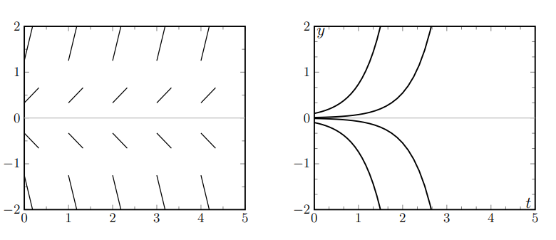
Consider the differential equation

\[\frac{d y}{d t}=2 y \]

Compute some of the slopes for various values of y and use this to sketch a slope field for this differential equation.

Solution

Equation (13.2.1) states that if a solution curve passes through a point \((t, y)\), then its tangent line at that point has a slope \(2 y\), regardless of the value of \(t\). This example is simple enough that we can state the following: for positive values of \(y\), the slope is positive; for negative values of \(y\), the slope is negative; and for \(y=0\), the slope is zero.

We provide some tabulated values of \(y\) indicating the values of the slope \(f(y)\), its sign, and what this implies about the local behavior of the solution and its direction. Then, in Figure \(13.1\) we combine this information to generate the direction field and the corresponding solution curves. Note that the direction of the arrows (rather than their absolute magnitude) provides the most important qualitative tendency for the slope field sketch.

Table 13.1: Table for the slope field diagram of differential equation (13.2.1), \(\frac{d y}{d t}=2 y\), described in Example 13.5.

\(\boldsymbol{y}\)	\(\boldsymbol{f}(\boldsymbol{y})\)	slope of tangent line	behavior of \(\boldsymbol{y}\)	direction of arrow
\(-2\)	\(-4\)	\(-\mathrm{ve}\)	decreasing	\(\searrow\)
\(-1\)	\(-2\)	\(-\mathrm{ve}\)	decreasing	\(\searrow\)
0	0	0	no change	\(\rightarrow\)
1	2	\(+\mathrm{ve}\)	increasing	\(\nearrow\)
2	4	\(+\mathrm{ve}\)	increasing	\(\nearrow\)

Figure 13.1: Direction field and solution curves for differential equation, \(\frac{d y}{d t}=2 y\) described in Example 13.5.

Mastered Material Check

14. Solve Differential Equation (13.4) analytically.

In constructing the slope field and solution curves, the following basic rules should be followed:

1. By convention, time flows from left to right along the \(t\) axis in our graphs, so the direction of all arrows (not usually indicated explicitly on the slope field) is always from left to right.
2. According to the differential equation, for any given value of the variable \(y\), the slope is given by the expression \(f(y)\) in the differential equation. The sign of that quantity is particularly important in determining whether the solution is locally increasing, decreasing, or neither. In the tables, we indicate this in the last column with the notation \(\nearrow, \searrow\), or \(\rightarrow\).
3. There is a single arrow at any point in the ty-plane, and consequently solution curves cannot intersect anywhere (although they can get arbitrarily close to one another).

We see some implications of these rules in our examples.

Example 13.6

Consider the differential equation

\[\frac{d y}{d t}=f(y)=y-y^{3} \]

Create a slope field diagram for this differential equation.

Solution

Based on the last example, we focus on the sign, rather than the value of the derivative \(f(y)\), since that sign determines whether the solutions increase, decrease, or stay constant. Recall that factoring helps to find zeros, and to identify where an expression changes sign. For example,

\[\frac{d y}{d t}=f(y)=y-y^{3}=y\left(1-y^{2}\right)=y(1+y)(1-y) . \nonumber \]

The sign of \(f\) depends on the signs of the factors \(y,(1+y),(1-y)\). For \(y<-1\), two factors, \(y,(1+y)\), are negative, whereas \((1-y)\) is positive, so that the product is positive overall. The sign of \(f(y)\) changes at each of the three points \(y=0, \pm 1\) where one or another of the three factors changes sign, as shown in Table 13.2. Eventually, to the right of all three (when \(y>1\) ), the sign is negative. We summarize these observations in Table \(13.2\) and show the slopes field and solution curves in Figure 13.2.

Table 13.2: Table for the slope field diagram of the \(\mathrm{DE}\) (13.5) described in Example 13.6.

\(\boldsymbol{y}\)	sign of \(f(y)\)	behavior of \(y\)	direction of arrow
\(y<-1\)	\(+\) ve	increasing	\(\nearrow\)
\(-1\)	0	no change	\(\rightarrow\)
\(-0.5\)	\(-\) ve	decreasing	\(\searrow\)
0	0	no change	\(\rightarrow\)
\(0.5\)	\(+\) ve	increasing	\(\nearrow\)
1	0	no change	\(\rightarrow\)
\(y>1\)	\(-\) ve	decreasing	\(\searrow\)

Figure 13.2: Direction field and solution curves for differential equation (13.5) described in Example 13.6.

A summary of steps in creating the slope field for Example 13.6.

Mastered Material Check

15. Graph the function \(f(y)=y(1+y)(1-y)\) and indiate where it changes sign.
16. Repeat the process for the function \(f(y)=y^{2}(1+y)^{2}(1-y)\)

Example 13.7

Sketch a slope field and solution curves for the problem of a cooling object, and specifically for

\[\frac{d T}{d t}=f(T)=0.2(10-T) \]

Solution

The family of curves shown in Figure \(13.3\) (also Figure 12.6) are solutions to (13.6). The function \(f(T)=0.2(10-T)\) corresponds to the slopes of tangent lines to these curves. We indicate the sign of \(f(T)\) and thereby the behavior of \(T(t)\) in Table 13.3. Note that there is only one change of sign, at \(T=10\). For smaller \(T\), the solution is always increasing and for larger \(T\), the solution is always decreasing. The slope field and solution curves are shown in Figure 13.3. In the slope field, one particular value of \(t\) is coloured to emphasize the associated changes in \(T\), as in Table 13.3.

Table 13.3: Table for the slope field diagram of \(\frac{d T}{d t}=0.2(10-T)\) described in Example \(13.7\).

\(\boldsymbol{T}\)	sign of \(f(T)\)	behavior of \(T\)	direction of arrow
\(T<10\)	\(+\) ve	increasing	\(\nearrow\)
\(T=10\)	0	no change	\(\rightarrow\)
\(T>10\)	-ve	decreasing	\(\searrow\)

Figure 13.3: Slope field and solution curves for a cooling object that satisfies the differential equation (13.6) in Example 13.7.

Mastered Material Check

17. Indicate the regions Figure \(13.3\) where \(T\) is increasing.
18. Where is \(T\) not changing in Figure 13.3?

We observe an agreement between the detailed solutions found analytically (Example 12.5), found using Euler’s method (Example 12.13), and those sketched using the new qualitative arguments (Example 13.7).

State-space diagrams

In Examples 13.5-13.7, we saw that we can understand qualitative features of solutions to the differential equation

\[\frac{d y}{d t}=f(y) \]

by examining the expression \(f(y)\). We used the sign of \(f(y)\) to assemble a slope field diagram and sketch solution curves. The slope field informed us about which initial values of \(y\) would increase, decrease or stay constant. We next show another way of determining the same information.

First, let us define a state space, also called phase line, which is essentially the \(y\)-axis with superimposed arrows representing the direction of flow.

Definition 13.2 (State space (or phase line))

A line representing the dependent variable (y) together with arrows to describe the flow along that line (increasing, decreasing, or stationary y) satisfying Equation (13.2.4) is called the state space diagram or the phase line diagram for the differential equation.

Rather than tabulating signs for \(f(y)\), we can arrive at similar conclusions by sketching \(f(y)\) and observing where this function is positive (implying that \(y\) increases) or negative ( \(y\) decreases). Places where \(f(y)=0\) ("zeros of \(f\) ") are important since these represent steady states ("static solutions", where there is no change in \(y\) ). Along the \(y\) axis (which is now on the horizontal axis of the sketch) increasing \(y\) means motion to the right, decreasing \(y\) means motion to the left.

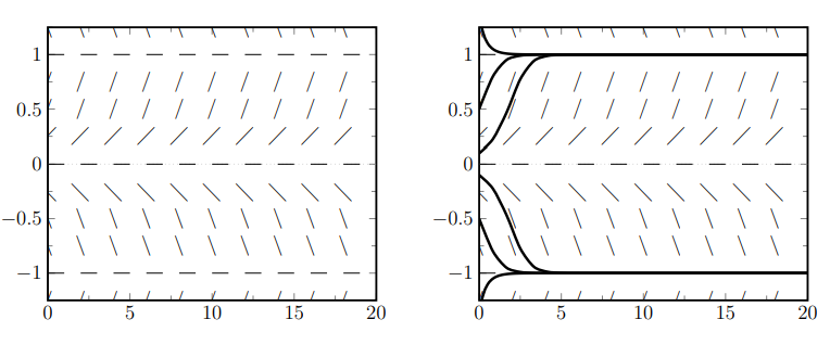
As we shall see, the information contained in this type of diagram provides a qualitative description of solutions to the differential equation, but with the explicit time behavior suppressed. This is illustrated by Figure 13.4, where we show the connection between the slope field diagram and the state space diagram for a typical differential equation.

Figure 13.4: The relationship of the slope field and state space diagrams. (a) A typical slope field. A few arrows have been added to indicate the direction of time flow along the tangent vectors. Now consider "looking down the time axis" as shown by the "eye" in this diagram. Then the \(t\) axis points towards us, and we see only the \(y\)-axis as in (b). Arrows on the \(y\)-axis indicate the directions of flow for various values of \(y\) as determined in (a). Now "rotate" the \(y\) axis so it is horizontal, as shown in (c). The direction of the arrows exactly correspond to places where \(f(y)\), in (c), is positive (which implies increasing \(y, \rightarrow\) ), or negative (which implies decreasing \(y, \leftarrow)\). The state space diagram is the \(y\)-axis in (b) or (c).

Example 13.8

Consider the differential equation

\[\frac{d y}{d t}=f(y)=y-y^{3} . \nonumber \]

Sketch \(f(y)\) versus y and use your sketch to determine where \(y\) is static, and where y increases or decreases. Then describe what this predicts starting from each of the three initial conditions:

1. \(y(0)=-0.5\),
2. \(y(0)=0.3\), or
3. \(y(0)=2\).

Solution

From Example 13.6, we know that \(f(y)=0\) at \(y=-1,0,1\). This means that \(y\) does not change at these steady state values, so, if we start a system off with \(y(0)=0\), or \(y(0)=\pm 1\), the value of \(y\) is static. The three places at which this happens are marked by heavy dots in Figure 13.5(a).

Figure 13.5: Steady states (dots) and intervals for which \(y\) increases or decreases for the differential equation (13.8).

We also see that \(f(y)<0\) for \(-1<y<0\) and for \(y>1\). In these intervals, \(y(t)\) must be a decreasing function of time \((d y / d t<0)\). On the other hand, for \(0<y<1\) or for \(y<-1\), we have \(f(y)>0\), so \(y(t)\) is increasing. See arrows on Figure 13.5(b). We see from this figure that there is a tendency for \(y\) to move away from the steady state value \(y=0\) and to approach either of the steady states at 1 or \(-1\). Starting from the initial values given above, we have

1. \(y(0)=-0.5\) results in \(y \rightarrow-1\),
2. \(y(0)=0.3\) leads to \(y \rightarrow 1\), and
3. \(y(0)=2\) implies \(y \rightarrow 1\).

Video explanation of the steps in the solution to Example 13.8. See Example \(13.8\).

Example 13.9 (A cooling object)

Sketch the same type of diagram for the problem of a cooling object and interpret its meaning.

Solution

Here, the differential equation is

\[\frac{d T}{d t}=f(T)=0.2(10-T) \]

A sketch of the rate of change, \(f(T)\) versus the temperature \(T\) is shown in Figure 13.6. We deduce the direction of the flow directly form this sketch.

Figure 13.6: Figure for Example 13.9, the differential equation (13.9).

Example 13.10

Create a similar qualitative sketch for the more general form of linear differential equation

\[\frac{d y}{d t}=f(y)=a-b y \]

For what values of \(y\) would there be no change?

Solution

The rate of change of \(y\) is given by the function \(f(y)=a-b y\). This is shown in Figure 13.7.

Figure 13.7: Qualitative sketch for Equation (13.10) in Example 13.10.

The steady state at which \(f(y)=0\) is at \(y=a / b\). Starting from an initial condition \(y(0)=a / b\), there would be no change. We also see from this figure that \(y\) approaches this value over time. After a long time, the value of \(y\) will be approximately \(a / b\).

Mastered Material Check

19. In Figures \(13.6\) and 13.7, where is the function positive?
20. Consider Equation (13.2.6) analytically: what value does \(y\) approach?

Steady states and stability

From the last few figures, we observe that wherever the function \(f\) on the right hand side of the differential equations crosses the horizontal axis (satisfies \(f=0\) ) there is a steady state. For example, in Figure \(13.6\) this takes place at \(T=10\). At that temperature the differential equation specifies that \(d T / d t=0\) and so, \(T=10\) is a steady state, a concept we first encountered in Chapter 12.

Definition 13.3 (Steady state)

A steady state is a state in which a system is not changing.

Example 13.11

Identify steady states of Equation (13.2.4),

\[\frac{d y}{d t}=y^{3}-y . \nonumber \]

Solution

Steady states are points that satisfy \(f(y)=0\). We already found those to be \(y=0\) and \(y=\pm 1\) in Example 13.8.

From Figure 13.5, we see that solutions starting close to \(y=1\) tend to get closer and closer to this value. We refer to this behavior as stability of the steady state.

Definition 13.4 (Stability)

We say that a steady state is stable if states that are initially close enough to that steady state will get closer to it with time. We say that a steady state is unstable, if states that are initially very close to it eventually move away from that steady state.

Example 13.12

Determine the stability of steady states of Equation (13.8):

\[\frac{d y}{d t}=y-y^{3} . \nonumber \]

Solution

From any starting value of \(y>0\) in this example, we see that after a long time, the solution curves tend to approach the value \(y=1\). States close to \(y=1\) get closer to it, so this is a stable steady state. For the steady state \(y=0\), we see that initial conditions near \(y=0\) move away over time. Thus, this steady state is unstable. Similarly, the steady state at \(y=-1\) is stable. In Figure \(13.5\) we show the stable steady states with black dots and the unstable steady state with an open dot.

Mastered Material Check

21. In the state space diagram in Figure 13.4, identify the stable steady states.