13.3: Applying qualitative analysis to biological models

Learning Objectives

1. Practice the techniques of slope field, state-space diagram, and steady state analysis on the logistic equation.
2. Explain the derivation of a model for interacting (healthy, infected) individuals based on a set of assumptions.
3. Identify that the resulting set of two ODEs can be reduced to a single ODE. Use qualitative methods to analyse the model behavior and to interpret the results.

The qualitative ideas developed so far will now be applied to to problems from biology. In the following sections we first use these methods to obtain a thorough understanding of logistic population growth. We then derive a model for the spread of a disease, and use qualitative arguments to analyze the predictions of that differential equation model.

Qualitative analysis of the logistic equation

We apply the new methods to the logistic equation.

Example 13.13

Find the steady states of the logistic equation, Eqn. (13.1.1):

\[\frac{d N}{d t}=r N \frac{(K-N)}{K} \nonumber \]

Solution

To determine the steady states of Equation (13.1), i.e. the level of population that would not change over time, we look for values of \(N\) such that

\[\frac{d N}{d t}=0 . \nonumber \]

This leads to

\[r N \frac{(K-N)}{K}=0, \nonumber \]

which has solutions \(N=0\) (no population at all) or \(N=K\) (the population is at its carrying capacity).

We could similarly find steady states of the scaled form of the logistic equation, Equation (13.1.3). Setting \(d y / d t=0\) leads to

\[0=\frac{d y}{d t}=r y(1-y) \quad \Rightarrow \quad y=0, \text { or } y=1 . \nonumber \]

This comes as no surprise since these values of \(y\) correspond to the values \(N=0\) and \(N=K\).

The scaled logistic equation, its slope field, and steady state values are discussed here.

A second way to analyze the scaled logistic equation, using the phase line approach, and its connection to the slope field method as described in Example 13.14.

Example 13.14

Draw a plot of the rate of change \(d y / d t\) versus the value of \(y\) for the scaled logistic equation, Equation (13.1.3):

\[\frac{d y}{d t}=r y(1-y) . \nonumber \]

Solution

In the plot of Figure \(13.8\) only \(y \geq 0\) is relevant. In the interval \(0<y<1\), the rate of change is positive, so that \(y\) increases, whereas for \(y>1\), the rate of change is negative, so \(y\) decreases. Since \(y\) refers to population size, we need not concern ourselves with behavior for \(y<0\).

From Figure \(13.8\) we deduce that solutions that start with a positive \(y\) value approach \(y=1\) with time. Solutions starting at either steady state \(y=0\) or \(y=1\) would not change. Restated in terms of the variable \(N(t)\), any initial population should approach its carrying capacity \(K\) with time.

Figure 13.8: Plot of \(d y / d t\) versus \(y\) for the the scaled logistic equation (13.1.3).

Mastered Material Check

22. Circle the steady states in Figure \(13.8\) and identify which one is stable.
23. Why is \(y<0\) not relevant in Example \(13.14 ?\)

We now look at the same equation from the perspective of the slope field.

Example 13.15

Draw a slope field for the scaled logistic equation with \(r=0.5\), that is for

\[\frac{d y}{d t}=f(y)=0.5 \cdot y(1-y) \]

Solution

We generate slopes for various values of \(y\) in Table \(13.4\) and plot the slope field in Figure 13.9(a).

Table 13.4: Table for slope field for the logistic equation (13.11). See Fig 13.9(a) for the resulting diagram.

\(\boldsymbol{y}\)	sign of \(f(y)\)	behavior of	direction of arrow
\(0\)	\(0\)	no change	\(\rightarrow\)
\(0<y<1\)	+ve	increasing	\(\nearrow\)
\(1\)	\(0\)	no change	\(\rightarrow\)
\(y>1\)	-ve	decreasing	\(\searrow\)

Figure 13.9: (a) Slope field and (b) solution curves for the logistic equation (13.11), \(\frac{d y}{d t}=0.5 \cdot y(1-y)\)

Finally, we practice Euler’s method to graph the numerical solution to Equation (13.11) from several initial conditions.

Example 13.16 (Numerical solutions to the logistic equation)

Use Euler’s method to approximate the solutions to the logistic equation (13.3.1).

Solution

In Figure 13.9(b) we show a set of solution curves, obtained by solving the equation numerically using Euler’s method. To obtain these solutions, a value of \(h=\Delta t=0.1\) was used. The solution is plotted for various initial conditions \(y(0)=y_{0}\). The successive values of \(y\) were calculated according to

\[y_{k+1}=y_{k}+0.5 y_{k}\left(1-y_{k}\right) h, \quad k=0, \ldots 100 . \nonumber \]

From Figure 13.9(b), we see that solution curves approach the steady state \(y=\) 1 , meaning that the population \(N(t)\) approaches the carrying capacity \(K\) for all positive starting values. A link to the spreadsheet that implements Euler’s method is included.

Mastered Material Check

24. What initial values \(y_{0}\) were used in drawing the different solution curves depicted in Figure 13.9(b)?

Link to Google Sheets. This spreadsheet implements Euler’s method for Example 13.16. A chart showing solutions from four initial conditions is included.

Example 13.17 (Inflection points)

Some of the curves shown in Figure \(13.9(b)\) have an inflection point, but others do not. Use the differential equation to determine which of the solution curves have an inflection point.

Solution

We have already established that all initial values in the range \(0<\) \(y_{0}<1\) are associated with increasing solutions \(y(t)\). Now we consider the concavity of those solutions. The logistic equation has the form

\[\frac{d y}{d t}=r y(1-y)=r y-r y^{2} \nonumber \]

Differentiate both sides using the chain rule and factor, to get

\[\frac{d^{2} y}{d t^{2}}=r \frac{d y}{d t}-2 r y \frac{d y}{d t}=r \frac{d y}{d t}(1-2 y) \nonumber \]

An inflection point would occur at places where the second derivative changes sign. This is possible for \(d y / d t=0\) or for \((1-2 y)=0\). We have already dismissed the first possibility because we argued that the rate of change is nonzero in the interval of interest. Thus we conclude that an inflection point would occur whenever \(y=1 / 2\). Any initial condition satisfying \(0<y_{0}<1 / 2\) would eventually pass through \(y=1 / 2\) on its way to the steady state level at \(y=1\), and in so doing, would have an inflection point.

Mastered Material Check

25. How do we know that initial conditions in the range \(0<y_{0}<1\) lead to increasing solutions?

A changing aphid population

In Chapters 1 and 5, we investigated a situation when predation and growth rates of an aphid population exactly balanced. But what happens if these two rates do not balance? We are now ready to tackle this question.

Featured Problem 13.1 (aphids): Consider the aphid-ladybug problem (Example 1.3) with aphid density \(x\), growth rate \(G(x)=r x\), and predation rate by a ladybug \(P(x)\) as in (1.10). (a) Write down a differential equation for the aphid population. (b) Use your equation, and a sketch of the two functions to answer the following question: What happens to the aphid population starting from various initial population sizes?

Hint: Growth rate (number of aphids born per unit time) contributes positively, whereas predation rate (number of aphids eaten per unit time) contributes negatively to the rate of change of aphids with respect to time (\(dx/dt\)).

The radius of a growing cell

In Section \(11.4\) we examined a cell in which nutrient absorption and consumption each contribute to changing the mass balance of the cell. We first wrote down a differential equation of the form

\[\frac{d m}{d t}=A-C . \nonumber \]

Assuming the cell was spherical, we showed that this equation results in the differential equation for the cell radius \(r(t)\) :

\[\frac{d r}{d t}=\frac{1}{\rho}\left(k_{1}-\frac{k_{2}}{3} r\right), \quad k_{1}, k_{2}, \rho>0 \nonumber \]

Using tools in this chapter, we can now understand what this implies about cell size growth.

Featured Problem 13.2 (How cell radius changes): Apply qualitative methods to Equation (13.12) so as to determine what happens to cells starting from various initial sizes. Is there a steady state cell size? How do your results compare to our findings in Section 1.2?

A model for the spread of a disease

In the era of human immunodeficiency virus (HIV), Severe Acute Respiratory Syndrome (SARS), Avian influenza ("bird flu") and similar emerging infectious diseases, it is prudent to consider how infection spreads, and how it could be controlled or suppressed. This motivates the following example.

For a given disease, let us subdivide the population into two classes: healthy individuals who are susceptible to catching the infection, and those that are currently infected and able to transmit the infection to others. We consider an infection that is mild enough that individuals recover at some constant rate, and that they become susceptible once recovered.

Note: usually, recovery from an illness leads to partial temporary immunity. While this, too, can be modelled, we restrict attention to the simpler case which is tractable using mathematics we have just introduced.

The simplest case to understand is that of a fixed population (with no birth, death or migration during the timescale of interest). A goal is to predict whether the infection spreads and persists (becomes endemic) in the population or whether it runs its course and disappear. We use the following notation:

\[\begin{aligned} & S(t)=\text { size of population of susceptible (healthy) individuals, } \\ & I(t)=\text { size of population of infected individuals, } \\ & N(t)=S(t)+I(t)=\text { total population size. } \end{aligned} \nonumber \]

We add a few simplifying assumptions.

1. The population mixes very well, so each individual is equally likely to contact and interact with any other individual. The contact is random.
2. Other than the state ( \(S\) or \(I\) ), individuals are "identical," with the same rates of recovery and infectivity.
3. On the timescale of interest, there is no birth, death or migration, only exchange between \(S\) and \(I\).

A video summary of the model for the spread of a disease, together with its analysis.

Example 13.18

Suppose that the process can be represented by the scheme

\[\begin{aligned} S+I & \rightarrow I+I, \\ I & \rightarrow S \end{aligned} \nonumber \]

The first part, transmission of disease from I to \(S\) involves interaction. The second part is recovery. Use the assumptions above to track the two populations and to formulate a set of differential equations for \(I(t)\) and \(S(t)\).

Solution

The following balance equations keeps track of individuals

\[\left[\begin{array}{c} \text { Rate of } \\ \text { change of } \\ I(t) \end{array}\right]=\left[\begin{array}{c} \text { Rate of gain } \\ \text { due to disease } \\ \text { transmission } \end{array}\right]-\left[\begin{array}{c} \text { Rate of loss } \\ \text { due to } \\ \text { recovery } \end{array}\right] \nonumber \]

According to our assumption, recovery takes place at a constant rate per unit time, denoted by \(\mu>0\). By the law of mass action, the disease transmission A video summary of the model for the spread of a disease, together with its analysis. rate should be proportional to the product of the populations, \((S \cdot I)\). Assigning \(\beta>0\) to be the constant of proportionality leads to the following differential equations for the infected population:

\[\frac{d I}{d t}=\beta S I-\mu I . \nonumber \]

Similarly, we can write a balance equation that tracks the population of susceptible individuals:

\[\left[\begin{array}{c} \text { Rate of } \\ \text { change of } \\ S(t) \end{array}\right]=-\left[\begin{array}{c} \text { Rate of Loss } \\ \text { due to disease } \\ \text { transmission } \end{array}\right]+\left[\begin{array}{c} \text { Rate of gain } \\ \text { due to } \\ \text { recovery } \end{array}\right] \nonumber \]

Observe that loss from one group leads to (exactly balanced) gain in the other group. By similar logic, the differential equation for \(S(t)\) is then

\[\frac{d S}{d t}=-\beta S I+\mu I . \nonumber \]

We have arrived at a system of equations that describe the changes in each of the groups,

\[\frac{d I}{d t}=\beta S I-\mu I\]

\[\frac{d S}{d t}=-\beta S I+\mu I\]

From Equations (13.3.2 and 13.3.3) it is clear that changes in one population depend on both, which means that the differential equations are coupled (linked to one another). Hence, we cannot "solve one" independently of the other. We must treat them as a pair. However, as we observe in the next examples, we can simplify this system of equations using the fact that the total population does not change.

Example 13.19

Use Equations(13.3.2 and 13.3.3) to show that the total population does not change (hint: show that the derivative of \(S(t)+I(t)\) is zero).

Solution

Add the equations to one another. Then we obtain

\[\frac{d}{d t}[I(t)+S(t)]=\frac{d I}{d t}+\frac{d S}{d t}=\beta S I-\mu I-\beta S I+\mu I=0 . \nonumber \]

Hence

\[\frac{d}{d t}[I(t)+S(t)]=\frac{d N}{d t}=0, \nonumber \]

which mean that \(N(t)=[I(t)+S(t)]=N=\) constant, so the total population does not change. (In Equation (13.1.1), here \(N\) is a constant and \(I(t), S(t)\) are the variables.)

Mastered Material Check

26. Identify any constants in Equations (13.3.2 and 13.3.3).
27. What are the units of those constants?
28. Why does the hint given in Example \(13.19\) help?

Video showing that the population \(N(t)=I(t)+S(t)\) is constant.

Example 13.20

Use the fact that \(N\) is constant to express \(S(t)\) in terms of \(I(t)\) and \(N\), and eliminate \(S(t)\) from the differential equation for \(I(t)\). Your equation should only contain the constants \(N, \beta, \mu\).

Solution

Since \(N=S(t)+I(t)\) is constant, we can write \(S(t)=N-I(t)\). Then, plugging this into the differential equation for \(I(t)\) we obtain

\[\frac{d I}{d t}=\beta S I-\mu I, \quad \Rightarrow \quad \frac{d I}{d t}=\beta(N-I) I-\mu I . \nonumber \]

Example 13.21

1. Show that the above equation can be written in the form \[\frac{d I}{d t}=\beta I(K-I), \nonumber \] where \(K\) is a constant.
2. Determine how this constant \(K\) depends on \(N, \beta\), and \(\mu\).
3. Is the constant \(K\) positive or negative?

Solution

a) We rewrite the differential equation for \(I(t)\) as follows:

\[\frac{d I}{d t}=\beta(N-I) I-\mu I=\beta I\left((N-I)-\frac{\mu}{\beta}\right)=\beta I\left(N-\frac{\mu}{\beta}-I\right) . \nonumber \]

b) We identify the constant,

\[K=\left(N-\frac{\mu}{\beta}\right) . \nonumber \]

c) Evidently, \(K\) could be either positive or negative, that is

\[\left\{\begin{array}{l} N \geq \frac{\mu}{\beta} \quad \Rightarrow K \geq 0 \\ N<\frac{\mu}{\beta} \quad \Rightarrow K<0 \end{array}\right. \nonumber \]

Using the above process, we have reduced the system of two differential equations for the two variables \(I(t), S(t)\) to a single differential equation for \(I(t)\), together with the statement \(S(t)=N-I(t)\). We now examine implications of this result using the qualitative methods of this chapter.

Mastered Material Check

29. Redo Example \(13.20\) but eliminate \(I(t)\) instead of \(S(t)\).
30. Analyze the equation you get for \(d S(t) / d t\) as done for \(d I / d t\) in Example 13.21.

Example 13.22

Consider the differential equation for \(I(t)\) given by

\[\frac{d I}{d t} \equiv f(I)=\beta I(K-I), \text { where } K=\left(N-\frac{\mu}{\beta}\right) \]

Find the steady states of the differential equation (13.14) and draw a state space diagram in each of the following cases:

1. \(K \geq 0\)
2. \(K<0\)

Use your diagram to determine which steady state(s) are stable or unstable.

Solution

Steady states of Equation (13.3.4) satisfy \(d I / d t=\beta I(K-I)=0\). Hence, these steady states are \(I=0\) (no infected individuals) and \(I=K\). The latter only makes sense if \(K \geq 0\). We plot the function \(f(I)=\beta I(K-I)\) in Equation (13.3.4) against the state variable \(I\) in Figure \(13.10\)

(a) for \(K \geq 0\) and

(b) for \(K<0\).

Figure 13.10: State-space diagrams for differential equation (13.14). Plots of \(f(I)\) as a function of \(I\) in the cases (a) \(K \geq 0\), and (b) \(K<0\). The grey regions are not biologically meaningful since \(I\) cannot be negative.

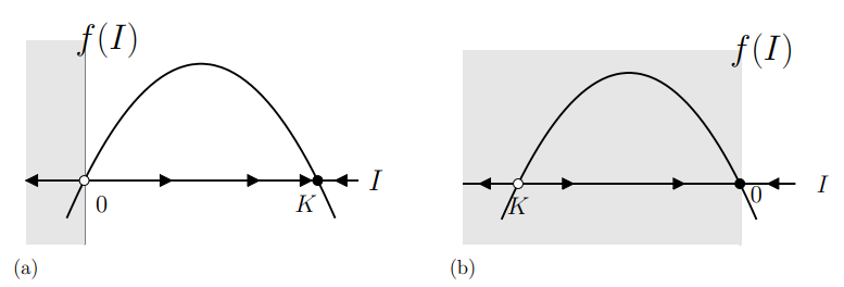
Since \(f(I)\) is quadratic in \(I\), its graph is a parabola and it opens downwards. We add arrows pointing right \((\rightarrow)\) in the regions where \(d I / d t>0\) and arrows pointing left \((\leftarrow)\) where \(d I / d t<0\).

In case (a), when \(K \geq 0\), we find that arrows point toward \(I=K\), so this steady state is stable. Arrows point away from \(I=0\), so this represents an unstable steady state.

In case (b), while we still have a parabolic graph with two steady states, the state \(I=K\) is not admissible since \(K\) is negative. Hence only one steady state, at \(I=0\) is relevant biologically, and all initial conditions move towards this state.

Mastered Material Check

31. What is the significance of the grey shaded regions in Figure 13.10.
32. Draw Figure \(13.10\) for \(K=0\).
33. Why is \(I=K\) not an admissible steady state if \(K<0\) ?

Example 13.23

Interpret the results of the model in terms of the disease, assuming that initially most of the population is in the susceptible \(S\) group, and a small number of infected individuals are present at \(t=0\).

Solution

In case (a), as long as the initial size of the infected group is positive ( \(I>0\) ), with time it approaches \(K\), that is, \(I(t) \rightarrow K=N-\mu / \beta\). The rest of the population is in the susceptible group, that is \(S(t) \rightarrow \mu / \beta\) (so that \(S(t)+I(t)=N\) is always constant.) This first scenario holds provided \(K>0\) which is equivalent to \(N>\mu / \beta\). There are then some infected and some healthy individuals in the population indefinitely, according to the model. In this case, we say that the disease becomes endemic.

In case (b), which corresponds to \(N<\mu / \beta\), we see that \(I(t) \rightarrow 0\) regardless of the initial size of the infected group. In that case, \(S(t) \rightarrow N\) so with time, the infected group shrinks and the healthy group grows so that the whole population becomes healthy. From these two results, we conclude that the disease is wiped out in a small population, whereas in a sufficiently large population, it can spread until a steady state is attained where some fraction of the population is always infected. In fact we have identified a threshold that separates these two behaviors:

\[\begin{aligned} & \frac{N \beta}{\mu}>1 \Rightarrow \text { disease becomes endemic, } \\ & \frac{N \beta}{\mu}<1 \Rightarrow \text { disease is wiped out. } \end{aligned} \nonumber \]

The ratio of constants in these inequalities, \(R_{0}=N \beta / \mu\) is called the basic reproduction number for the disease. Many current and much more detailed models for disease transmission also have such threshold behavior, and the ratio that determines whether the disease spreads or disappears, \(R_{0}\) is of great interest in vaccination strategies. This ratio represents the number of infections that arise when 1 infected individual interacts with a population of \(N\) susceptible individuals.

Mastered Material Check

34. In the case that \(\beta=0.001\) per person per day and \(\mu=0.1\) per day, how large would the population have to be for the disease to become endemic?
35. Frequent hand-washing can be a protective measure that decreases the spread of disease. Which parameter of the model would this affect and in what way?

A video summarizing the interpretation of the model and the meaning of the constant \(R_{0}=N \beta / \mu\).