
13.4: Summary
- Page ID
- 121154

\( \newcommand{\vecs}[1]{\overset { \scriptstyle \rightharpoonup} {\mathbf{#1}} } \)
\( \newcommand{\vecd}[1]{\overset{-\!-\!\rightharpoonup}{\vphantom{a}\smash {#1}}} \)
\( \newcommand{\id}{\mathrm{id}}\) \( \newcommand{\Span}{\mathrm{span}}\)
( \newcommand{\kernel}{\mathrm{null}\,}\) \( \newcommand{\range}{\mathrm{range}\,}\)
\( \newcommand{\RealPart}{\mathrm{Re}}\) \( \newcommand{\ImaginaryPart}{\mathrm{Im}}\)
\( \newcommand{\Argument}{\mathrm{Arg}}\) \( \newcommand{\norm}[1]{\| #1 \|}\)
\( \newcommand{\inner}[2]{\langle #1, #2 \rangle}\)
\( \newcommand{\Span}{\mathrm{span}}\)
\( \newcommand{\id}{\mathrm{id}}\)
\( \newcommand{\Span}{\mathrm{span}}\)
\( \newcommand{\kernel}{\mathrm{null}\,}\)
\( \newcommand{\range}{\mathrm{range}\,}\)
\( \newcommand{\RealPart}{\mathrm{Re}}\)
\( \newcommand{\ImaginaryPart}{\mathrm{Im}}\)
\( \newcommand{\Argument}{\mathrm{Arg}}\)
\( \newcommand{\norm}[1]{\| #1 \|}\)
\( \newcommand{\inner}[2]{\langle #1, #2 \rangle}\)
\( \newcommand{\Span}{\mathrm{span}}\) \( \newcommand{\AA}{\unicode[.8,0]{x212B}}\)
\( \newcommand{\vectorA}[1]{\vec{#1}} % arrow\)
\( \newcommand{\vectorAt}[1]{\vec{\text{#1}}} % arrow\)
\( \newcommand{\vectorB}[1]{\overset { \scriptstyle \rightharpoonup} {\mathbf{#1}} } \)
\( \newcommand{\vectorC}[1]{\textbf{#1}} \)
\( \newcommand{\vectorD}[1]{\overrightarrow{#1}} \)
\( \newcommand{\vectorDt}[1]{\overrightarrow{\text{#1}}} \)
\( \newcommand{\vectE}[1]{\overset{-\!-\!\rightharpoonup}{\vphantom{a}\smash{\mathbf {#1}}}} \)
\( \newcommand{\vecs}[1]{\overset { \scriptstyle \rightharpoonup} {\mathbf{#1}} } \)
\( \newcommand{\vecd}[1]{\overset{-\!-\!\rightharpoonup}{\vphantom{a}\smash {#1}}} \)
- A differential equation of the form \(\alpha \frac{d y}{d t}+\beta y+\gamma=0\) is linear (and "first order"). We encountered several examples of nonlinear DEs in this chapter.
- A (possibly nonlinear) differential equation \(\frac{d y}{d t}=f(y)\) can be analyzed qualitatively by observing where \(f(y)\) is positive, negative or zero.
- A slope field (or "direction field") is a collection of tangent vectors for solutions to a differential equation. Slope fields can be sketched from \(f(y)\) without the need to solve the differential equation.
- A solution curve drawn in a slope field corresponds to a single solution to a differential equation, with some initial \(y_{0}\) value given.
- A state space (or "phase line" diagram) for the differential equation is a \(y\) axis, together with arrows describing the flow (increasing/decreasing/stationary) along that axis. It can be obtained from a sketch of \(f(y)\).
- A steady state is stable if nearby states get closer. A steady state is unstable if nearby states get further away with time.
- Creating/interpreting slope field and state space diagrams is helpful in understanding the behavior of solutions to differential equations.
- Applications considered in this chapter included:
- the logistic equations for population growth (a nonlinear differential equation, scaling, steady state and slope field demonstration);
- the Law of Mass Action (a nonlinear differential equation);
- a cooling object (state space and phase line diagram demonstration); and
- disease spread model (an extensive exposition on qualitative differential equation methods).
- Why is it helpful to rescale an equation?
- Identify which of the following differential equations are linear:
- \(5 \frac{d y}{d t}-y=-0.5\)
- \(\left(\frac{d y}{d t}\right)^{2}+y+1=0\)
- \(\frac{d y}{d x}+\pi y+\rho=3\)
- \(\frac{d x}{d t}+x+2=-3 x\)
- Consider the following slope field:
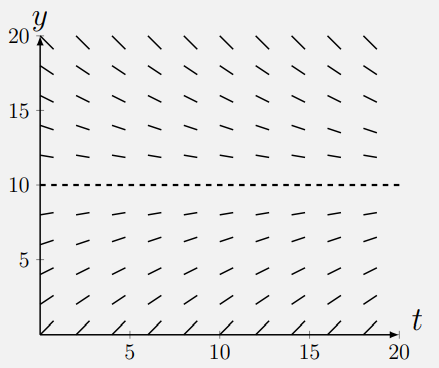
- Where is \(y\) decreasing?
- What is \(y\) approaching?
- Circle the stable steady states in the following state space diagram