8.E: Differential Equations (Exercises)

8.1: Basics of Differential Equations

In exercises 1 - 7, determine the order of each differential equation.

1) \( y′+y=3y^2\)

Answer

1st-order

2) \( (y′)^2=y′+2y\)

3) \( y'''+y''y′=3x^2\)

Answer

3rd-order

4) \( y′=y''+3t^2\)

5) \( \dfrac{dy}{dt}=t\)

Answer

1st-order

6) \( \dfrac{dy}{dx}+\dfrac{d^2y}{dx^2}=3x^4\)

7) \(\left(\dfrac{dy}{dt}\right)^2+8\dfrac{dy}{dt}+3y=4t\)

Answer

1st-order

In exercises 8 - 17, verify that the given function is a solution to the given differential equation.

8) \( y=\dfrac{x^3}{3}\quad\) solves \(\quad y′=x^2\)

9) \( y=2e^{−x}+x−1\quad\) solves \(\quad y′=x−y\)

10) \( y=e^{3x}−\dfrac{e^x}{2}\quad\) solves \(\quad y′=3y+e^x\)

11) \( y=\dfrac{1}{1−x}\quad\) solves \(\quad y′=y^2\)

12) \( y=e^{x^2}/2\quad\) solves \(\quad y′=xy\)

13) \( y=4+\ln x\quad\) solves \(\quad xy′=1\)

14) \( y=3−x+x\ln x\quad\) solves \(\quad y′=\ln x\)

15) \( y=2e^x−x−1\quad\) solves \(\quad y′=y+x\)

16) \( y=e^x+\dfrac{\sin x}{2}−\dfrac{\cos x}{2}\quad\) solves \(\quad y′=\cos x+y\)

17) \( y=πe^{−\cos x}\quad\) solves \(\quad y′=y\sin x\)

In exercises 18 - 27, verify the given general solution and find the particular solution.

18) Find the particular solution to the differential equation \( y′=4x^2\) that passes through \( (−3,−30)\), given that \( y=C+\dfrac{4x^3}{3}\) is a general solution.

19) Find the particular solution to the differential equation \( y′=3x^3\) that passes through \( (1,4.75)\), given that \( y=C+\dfrac{3x^4}{4}\) is a general solution.

Answer

\( y=4+\dfrac{3x^4}{4}\)

20) Find the particular solution to the differential equation \( y′=3x^2y\) that passes through \( (0,12)\), given that \( y=Ce^{x^3}\) is a general solution.

21) Find the particular solution to the differential equation \( y′=2xy\) that passes through \( (0,\frac{1}{2})\), given that \( y=Ce^{x^2}\) is a general solution.

Answer

\( y=\frac{1}{2}e^{x^2}\)

22) Find the particular solution to the differential equation \( y′=(2xy)^2\) that passes through \( (1,−\frac{1}{2})\), given that \( y=−\dfrac{3}{C+4x^3}\) is a general solution.

23) Find the particular solution to the differential equation \( y′x^2=y\) that passes through \( (1,\frac{2}{e})\), given that \( y=Ce^{−1/x}\) is a general solution.

Answer

\( y=2e^{−1/x}\)

24) Find the particular solution to the differential equation \( 8\dfrac{dx}{dt}=−2\cos(2t)−\cos(4t)\) that passes through \( (π,π)\), given that \( x=C−\frac{1}{8}\sin(2t)−\frac{1}{32}\sin(4t)\) is a general solution.

25) Find the particular solution to the differential equation \( \dfrac{du}{dt}=\tan u\) that passes through \( (1,\frac{π}{2})\), given that \( u=\sin^{−1}(e^{C+t})\) is a general solution.

Answer

\( u=\sin^{−1}(e^{−1+t})\)

26) Find the particular solution to the differential equation \( \dfrac{dy}{dt}=e^{(t+y)}\) that passes through \( (1,0)\), given that \( y=−\ln(C−e^t)\) is a general solution.

27) Find the particular solution to the differential equation \( y′(1−x^2)=1+y\) that passes through \( (0,−2),\) given that \( y=C\dfrac{\sqrt{x+1}}{\sqrt{1−x}}−1\) is a general solution.

Answer

\( y=−\dfrac{\sqrt{x+1}}{\sqrt{1−x}}−1\)

In exercises 28 - 37, find the general solution to the differential equation.

28) \( y′=3x+e^x\)

29) \( y′=\ln x+\tan x\)

Answer

\( y=C−x+x\ln x−\ln(\cos x)\)

30) \( y′=\sin x e^{\cos x}\)

31) \( y′=4^x\)

Answer

\( y=C+\dfrac{4^x}{\ln(4)}\)

32) \( y′=\sin^{−1}(2x)\)

33) \( y′=2t\sqrt{t^2+16}\)

Answer

\( y=\frac{2}{3}\sqrt{t^2+16}(t^2+16)+C\)

34) \( x′=\coth t+\ln t+3t^2\)

35) \( x′=t\sqrt{4+t}\)

Answer

\( x=\frac{2}{15}\sqrt{4+t}(3t^2+4t−32)+C\)

36) \( y′=y\)

37) \( y′=\dfrac{y}{x}\)

Answer

\( y=Cx\)

In exercises 38 - 42, solve the initial-value problems starting from \( y(t=0)=1\) and \( y(t=0)=−1.\) Draw both solutions on the same graph.

38) \( \dfrac{dy}{dt}=2t\)

39) \( \dfrac{dy}{dt}=−t\)

Answer

\( y=1−\dfrac{t^2}{2},\) and \(y=−\dfrac{t^2}{2}−1\)

40) \( \dfrac{dy}{dt}=2y\)

41) \( \dfrac{dy}{dt}=−y\)

Answer

\( y=e^{−t}\) and \(y=−e^{−t}\)

42) \( \dfrac{dy}{dt}=2\)

In exercises 43 - 47, solve the initial-value problems starting from \( y_0=10\). At what time does \(y\) increase to \(100\) or drop to \(1\)?

43) \( \dfrac{dy}{dt}=4t\)

Answer

\( y=2(t^2+5),\) When \(t=3\sqrt{5},\) \(y\) will increase to \(100\).

44) \( \dfrac{dy}{dt}=4y\)

45) \( \dfrac{dy}{dt}=−2y\)

Answer

\( y=10e^{−2t},\) When \(t=−\frac{1}{2}\ln(\frac{1}{10}),\) \(y\) will decrease to \(1\).

46) \( \dfrac{dy}{dt}=e^{4t}\)

47) \( \dfrac{dy}{dt}=e^{−4t}\)

Answer

\( y=\frac{1}{4}(41−e^{−4t}),\) Neither condition will ever happen.

Recall that a family of solutions includes solutions to a differential equation that differ by a constant. For exercises 48 - 52, use your calculator to graph a family of solutions to the given differential equation. Use initial conditions from \( y(t=0)=−10\) to \( y(t=0)=10\) increasing by \( 2\). Is there some critical point where the behavior of the solution begins to change?

48) [T] \( y′=y(x)\)

49) [T] \( xy′=y\)

Answer

Solution changes from increasing to decreasing at \( y(0)=0\).

50) [T] \( y′=t^3\)

51) [T] \( y′=x+y\) (Hint: \( y=Ce^x−x−1\) is the general solution)

Answer

Solution changes from increasing to decreasing at \( y(0)=0\).

52) [T] \( y′=x\ln x+\sin x\)

53) Find the general solution to describe the velocity of a ball of mass \( 1\) lb that is thrown upward at a rate of \( a\) ft/sec.

Answer

\( v(t)=−32t+a\)

54) In the preceding problem, if the initial velocity of the ball thrown into the air is \( a=25\) ft/s, write the particular solution to the velocity of the ball. Solve to find the time when the ball hits the ground.

55) You throw two objects with differing masses \( m_1\) and \( m_2\) upward into the air with the same initial velocity of \( a\) ft/s. What is the difference in their velocity after \( 1\) second?

Answer

\( 0\) ft/s

56) [T] You throw a ball of mass \( 1\) kilogram upward with a velocity of \( a=25\) m/s on Mars, where the force of gravity is \( g=−3.711\) m/s². Use your calculator to approximate how much longer the ball is in the air on Mars.

57) [T] For the previous problem, use your calculator to approximate how much higher the ball went on Mars.

Answer

\( 4.86\) meters

58) [T] A car on the freeway accelerates according to \( a=15\cos(πt),\) where \( t\) is measured in hours. Set up and solve the differential equation to determine the velocity of the car if it has an initial speed of \( 51\) mph. After \( 40\) minutes of driving, what is the driver’s velocity?

59) [T] For the car in the preceding problem, find the expression for the distance the car has traveled in time \( t\), assuming an initial distance of \( 0\). How long does it take the car to travel \( 100\) miles? Round your answer to hours and minutes.

Answer

\( x=50t−\frac{15}{π^2}\cos(πt)+\frac{3}{π^2},2\) hours \( 1\) minute

60) [T] For the previous problem, find the total distance traveled in the first hour.

61) Substitute \( y=Be^{3t}\) into \( y′−y=8e^{3t}\) to find a particular solution.

Answer

\( y=4e^{3t}\)

62) Substitute \( y=a\cos(2t)+b\sin(2t)\) into \( y′+y=4\sin(2t)\) to find a particular solution.

63) Substitute \( y=a+bt+ct^2\) into \( y′+y=1+t^2\) to find a particular solution.

Answer

\( y=1−2t+t^2\)

64) Substitute \( y=ae^t\cos t+be^t\sin t\) into \( y′=2e^t\cos t\) to find a particular solution.

65) Solve \( y′=e^{kt}\) with the initial condition \( y(0)=0\) and solve \( y′=1\) with the same initial condition. As \( k\) approaches \( 0\), what do you notice?

Answer

\( y=\frac{1}{k}(e^{kt}−1)\) and \( y=t\)

8.2: Direction Fields and Numerical Methods

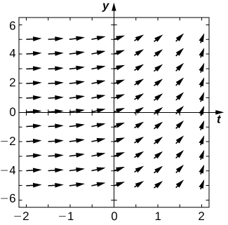
For the following problems, use the direction field below from the differential equation \(\displaystyle y'=−2y.\) Sketch the graph of the solution for the given initial conditions.

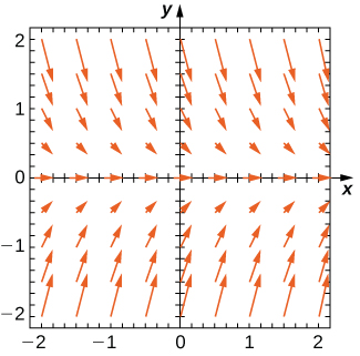
1) \(\displaystyle y(0)=1\)

2) \(\displaystyle y(0)=0\)

Solution:

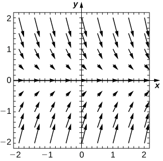
3) \(\displaystyle y(0)=−1\)

4) Are there any equilibria? What are their stabilities?

Solution: \(\displaystyle y=0\) is a stable equilibrium

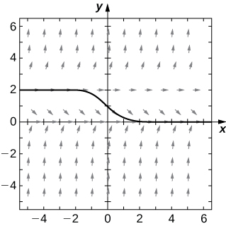
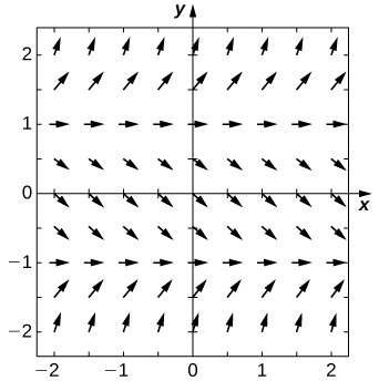
For the following problems, use the direction field below from the differential equation \(\displaystyle y'=y^2−2y\). Sketch the graph of the solution for the given initial conditions.

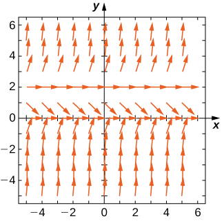
5) \(\displaystyle y(0)=3\)

6) \(\displaystyle y(0)=1\)

Solution:

7) \(\displaystyle y(0)=−1\)

8) Are there any equilibria? What are their stabilities?

Solution: \(\displaystyle y=0\) is a stable equilibrium and \(\displaystyle y=2\) is unstable

Draw the direction field for the following differential equations, then solve the differential equation. Draw your solution on top of the direction field. Does your solution follow along the arrows on your direction field?

9) \(\displaystyle y'=t^3\)

10) \(\displaystyle y'=e^t\)

11) \(\displaystyle \frac{dy}{dx}=x^2cosx\)

12) \(\displaystyle \frac{dy}{dt}=te^t\)

13) \(\displaystyle \frac{dx}{dt}=cosh(t)\)

Draw the directional field for the following differential equations. What can you say about the behavior of the solution? Are there equilibria? What stability do these equilibria have?

14) \(\displaystyle y'=y^2−1\)

Solution:

15) \(\displaystyle y'=y−x\)

16) \(\displaystyle y'=1−y^2−x^2\)

Solution:

17) \(\displaystyle y'=t^2siny\)

18) \(\displaystyle y'=3y+xy\)

Solution:

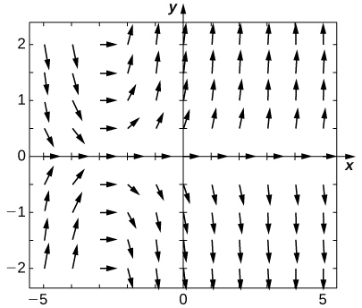
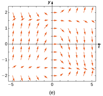
Match the direction field with the given differential equations. Explain your selections.

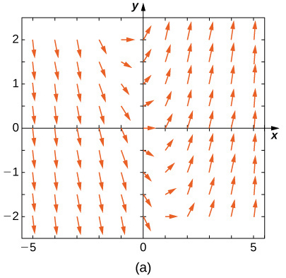
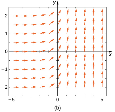
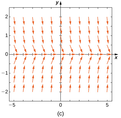
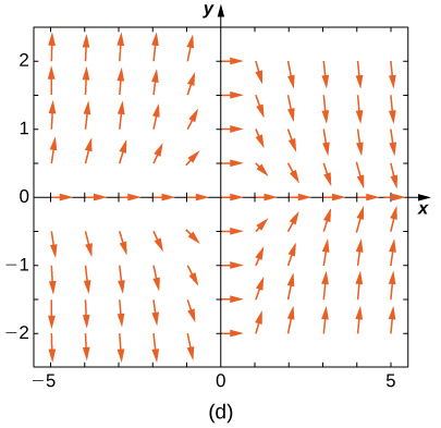
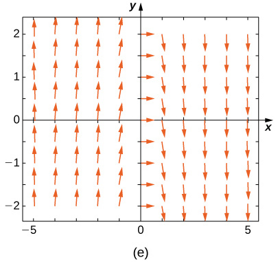
19) \(\displaystyle y'=−3y\)

20) \(\displaystyle y'=−3t\)

Solution: \(\displaystyle E\)

21) \(\displaystyle y'=e^t\)

22) \(\displaystyle y'=\frac{1}{2}y+t\)

Solution: \(\displaystyle A\)

23) \(\displaystyle y'=−ty\)

Match the direction field with the given differential equations. Explain your selections.

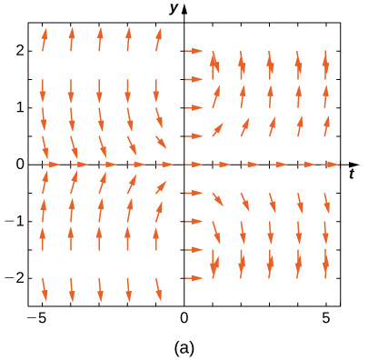
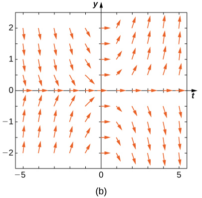
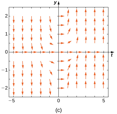
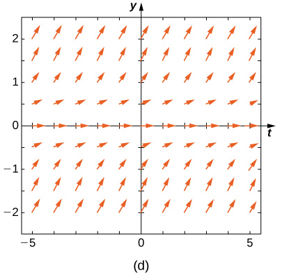
24) \(\displaystyle y'=tsiny\)

Solution: \(\displaystyle B\)

25) \(\displaystyle y'=−tcosy\)

26) \(\displaystyle y'=ttany\)

Solution: \(\displaystyle A\)

27) \(\displaystyle y'=sin^2y\)

28) \(\displaystyle y'=y^2t^3\)

Solution: \(\displaystyle C\)

Estimate the following solutions using Euler’s method with \(\displaystyle n=5\) steps over the interval \(\displaystyle t=[0,1].\) If you are able to solve the initial-value problem exactly, compare your solution with the exact solution. If you are unable to solve the initial-value problem, the exact solution will be provided for you to compare with Euler’s method. How accurate is Euler’s method?

29) \(\displaystyle y'=−3y,y(0)=1\)

30) \(\displaystyle y'=t^2\)

Solution: \(\displaystyle 2.24,\) exact: \(\displaystyle 3\)

31) \(\displaystyle y′=3t−y,y(0)=1.\) Exact solution is \(\displaystyle y=3t+4e^{−t}−3\)

32) \(\displaystyle y′=y+t^2,y(0)=3.\) Exact solution is \(\displaystyle y=5e^t−2−t^2−2t\)

Solution: \(\displaystyle 7.739364,\) exact: \(\displaystyle 5(e−1)\)

33) \(\displaystyle y′=2t,y(0)=0\)

34) [T] \(\displaystyle y'=e^{(x+y)},y(0)=−1.\) Exact solution is \(\displaystyle y=−ln(e+1−e^x)\)

Solution: \(\displaystyle −0.2535\) exact: \(\displaystyle 0\)

35) \(\displaystyle y′=y^2ln(x+1),y(0)=1.\) Exact solution is \(\displaystyle y=−\frac{1}{(x+1)(ln(x+1)−1)}\)

36) \(\displaystyle y′=2^x,y(0)=0,\) Exact solution is \(\displaystyle y=\frac{2^x−1}{ln(2)}\)

Solution: \(\displaystyle 1.345,\) exact: \(\displaystyle \frac{1}{ln(2)}\)

37) \(\displaystyle y′=y,y(0)=−1.\) Exact solution is \(\displaystyle y=−e^x\).

38) \(\displaystyle y′=−5t,y(0)=−2.\) Exact solution is \(\displaystyle y=−\frac{5}{2}t^2−2\)

Solution: \(\displaystyle −4,\) exact: \(\displaystyle −1/2\)

Differential equations can be used to model disease epidemics. In the next set of problems, we examine the change of size of two sub-populations of people living in a city: individuals who are infected and individuals who are susceptible to infection. \(\displaystyle S\) represents the size of the susceptible population, and \(\displaystyle I\) represents the size of the infected population. We assume that if a susceptible person interacts with an infected person, there is a probability \(\displaystyle c\) that the susceptible person will become infected. Each infected person recovers from the infection at a rate \(\displaystyle r\) and becomes susceptible again. We consider the case of influenza, where we assume that no one dies from the disease, so we assume that the total population size of the two sub-populations is a constant number, \(\displaystyle N\). The differential equations that model these population sizes are

\(\displaystyle S'=rI−cSI\) and \(\displaystyle I'=cSI−rI.\)

Here \(\displaystyle c\) represents the contact rate and \(\displaystyle r\) is the recovery rate.

39) Show that, by our assumption that the total population size is constant \(\displaystyle (S+I=N),\) you can reduce the system to a single differential equation in \(\displaystyle I:I'=c(N−I)I−rI.\)

40) Assuming the parameters are \(\displaystyle c=0.5,N=5,\) and \(\displaystyle r=0.5\), draw the resulting directional field.

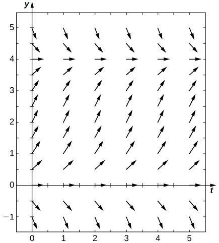
41) [T] Use computational software or a calculator to compute the solution to the initial-value problem \(\displaystyle y'=ty,y(0)=2\) using Euler’s Method with the given step size \(\displaystyle h\). Find the solution at \(\displaystyle t=1\). For a hint, here is “pseudo-code” for how to write a computer program to perform Euler’s Method for \(\displaystyle y'=f(t,y),y(0)=2:\)

Create function \(\displaystyle f(t,y)\)

Define parameters \(\displaystyle y(1)=y_0,t(0)=0,\) step size \(\displaystyle h\), and total number of steps, \(\displaystyle N\)

Write a for loop:

for \(\displaystyle k=1\) to \(\displaystyle N\)

\(\displaystyle fn=f(t(k),y(k))\)

\(\displaystyle y(k+1)=y(k)+h*fn\)

\(\displaystyle t(k+1)=t(k)+h\)

42) Solve the initial-value problem for the exact solution.

Solution: \(\displaystyle y'=2e^{t^2/2}\)

43) Draw the directional field

44) \(\displaystyle h=1\)

Solution: \(\displaystyle 2\)

45) [T] \(\displaystyle h=10\)

46) [T] \(\displaystyle h=100\)

Solution: \(\displaystyle 3.2756\)

47) [T] \(\displaystyle h=1000\)

48) [T] Evaluate the exact solution at \(\displaystyle t=1\). Make a table of errors for the relative error between the Euler’s method solution and the exact solution. How much does the error change? Can you explain?

Solution: \(\displaystyle 2\sqrt{e}\)

Step Size	Error
\(\displaystyle h=1\)	\(\displaystyle 0.3935\)
\(\displaystyle h=10\)	\(\displaystyle 0.06163\)
\(\displaystyle h=100\)	\(\displaystyle 0.006612\)
\(\displaystyle h=10000\)	\(\displaystyle 0.0006661\)

Consider the initial-value problem \(\displaystyle y'=−2y,y(0)=2.\)

49) Show that \(\displaystyle y=2e^{−2x}\) solves this initial-value problem.

50) Draw the directional field of this differential equation.

Solution:

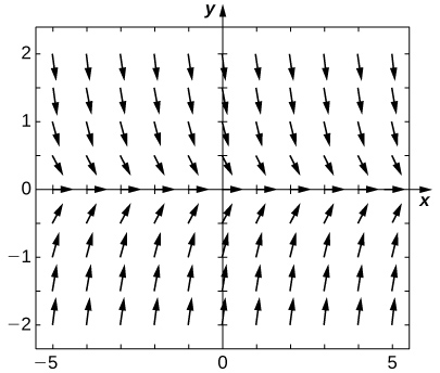
51) [T] By hand or by calculator or computer, approximate the solution using Euler’s Method at \(\displaystyle t=10\) using \(\displaystyle h=5\).

52) [T] By calculator or computer, approximate the solution using Euler’s Method at \(\displaystyle t=10\) using \(\displaystyle h=100.\)

Solution: \(\displaystyle 4.0741e^{−10}\)

53) [T] Plot exact answer and each Euler approximation (for \(\displaystyle h=5\) and \(\displaystyle h=100\)) at each h on the directional field. What do you notice?

8.3: Separable Equations

In exercises 1 - 4, solve the following initial-value problems with the initial condition \( y_0=0\) and graph the solution.

1) \( \dfrac{dy}{dt}=y+1\)

Answer

\( y=e^t−1\)

2) \( \dfrac{dy}{dt}=y−1\)

3) \( \dfrac{dy}{dt}=-y+1\)

Answer

\( y=1−e^{−t}\)

4) \( \dfrac{dy}{dt}=−y−1\)

In exercises 5 - 14, find the general solution to the differential equation.

5) \( x^2y'=(x+1)y\)

Answer

\( y=Cxe^{−1/x}\)

6) \( y'=\tan(y)x\)

7) \( y'=2xy^2\)

Answer

\( y=\dfrac{1}{C−x^2}\)

8) \( \dfrac{dy}{dt}=y\cos(3t+2)\)

9) \( 2x\dfrac{dy}{dx}=y^2\)

Answer

\( y=−\dfrac{2}{C+\ln|x|}\)

Solution:

10) \( y'=e^yx^2\)

11) \( (1+x)y'=(x+2)(y−1)\)

Answer

\( y=Ce^x(x+1)+1\)

12) \( \dfrac{dx}{dt}=3t^2(x^2+4)\)

13) \( t\dfrac{dy}{dt}=\sqrt{1−y^2}\)

Answer

\( y=\sin(\ln|t|+C)\)

14) \( y'=e^xe^y\)

In exercises 15 - 24, find the solution to the initial-value problem.

15) \( y'=e^{y−x}, \quad y(0)=0\)

Answer

\( y=−\ln(e^{−x})\) which simplifies to \(y = x\)

16) \( y'=y^2(x+1), \quad y(0)=2\)

17) \( \dfrac{dy}{dx}=y^3xe^{x^2}, \quad y(0)=1\)

Answer

\( y=\dfrac{1}{\sqrt{2−e^{x^2}}}\)

18) \( \dfrac{dy}{dt}=y^2e^x\sin(3x), \quad y(0)=1\)

19) \( y'=\dfrac{x}{\text{sech}^2y}, \quad y(0)=0\)

Answer

\( y=\tanh^{−1}\left(\dfrac{x^2}{2}\right)\)

20) \( y'=2xy(1+2y), \quad y(0)=−1\)

21) \( \dfrac{dx}{dt}=\ln(t)\sqrt{1−x^2}, \quad x(1)=0\)

Answer

\( x=\sin(1 - t + t\ln t)\)

22) \( y'=3x^2(y^2+4),\quad y(0)=0\)

23) \( y'=e^y5^x, \quad y(0)=\ln(\ln(5))\)

Answer

\( y=\ln(\ln(5))−\ln(2−5^x)\)

24) \( y'=−2x\tan(y), \quad y(0)=\dfrac{π}{2}\)

For problems 25 - 29, use a software program or your calculator to generate the directional fields. Solve explicitly and draw solution curves for several initial conditions. Are there some critical initial conditions that change the behavior of the solution?

25) [T] \( y'=1−2y\)

Answer

\( y=Ce^{−2}x+\dfrac{1}{2}\)

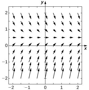
26) [T] \( y'=y^2x^3\)

27) [T] \( y'=y^3e^x\)

Answer

\( y=\dfrac{1}{\sqrt{2}\sqrt{C−e^x}}\)

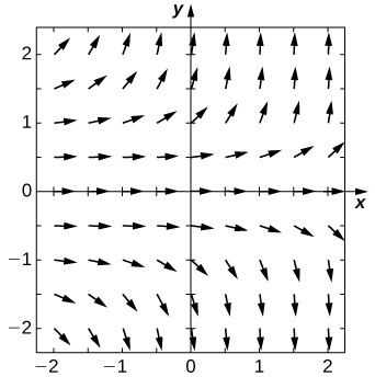
28) [T] \( y'=e^y\)

29) [T] \( y'=y\ln(x)\)

Answer

\( y=Ce^{−x}x^x\)

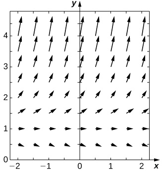
30) Most drugs in the bloodstream decay according to the equation \( y'=cy\), where \( y\) is the concentration of the drug in the bloodstream. If the half-life of a drug is \( 2\) hours, what fraction of the initial dose remains after \( 6\) hours?

31) A drug is administered intravenously to a patient at a rate \( r\) mg/h and is cleared from the body at a rate proportional to the amount of drug still present in the body, \( d\) Set up and solve the differential equation, assuming there is no drug initially present in the body.

Answer

\( y=\frac{r}{d}(1−e^{−dt})\)

32) [T] How often should a drug be taken if its dose is \( 3\) mg, it is cleared at a rate \( c=0.1\) mg/h, and \( 1\) mg is required to be in the bloodstream at all times?

33) A tank contains \( 1\) kilogram of salt dissolved in \( 100\) liters of water. A salt solution of \( 0.1\) kg salt/L is pumped into the tank at a rate of \( 2\) L/min and is drained at the same rate. Solve for the salt concentration at time \( t\). Assume the tank is well mixed.

Answer

\( y(t)=10−9e^{−t/50}\)

34) A tank containing \( 10\) kilograms of salt dissolved in \( 1000\) liters of water has two salt solutions pumped in. The first solution of \( 0.2\) kg salt/L is pumped in at a rate of \( 20\) L/min and the second solution of \( 0.05\) kg salt/L is pumped in at a rate of \( 5\) L/min. The tank drains at \( 25\) L/min. Assume the tank is well mixed. Solve for the salt concentration at time \( t\).

35) [T] For the preceding problem, find how much salt is in the tank \( 1\) hour after the process begins.

Answer

\( 134.3\) kilograms

36) Torricelli’s law states that for a water tank with a hole in the bottom that has a cross-section of \( A\) and with a height of water \( h\) above the bottom of the tank, the rate of change of volume of water flowing from the tank is proportional to the square root of the height of water, according to \( \dfrac{dV}{dt}=−A\sqrt{2gh}\), where \( g\) is the acceleration due to gravity. Note that \( \dfrac{dV}{dt}=A\dfrac{dh}{dt}\). Solve the resulting initial-value problem for the height of the water, assuming a tank with a hole of radius \( 2\) ft. The initial height of water is \( 100\) ft.

37) For the preceding problem, determine how long it takes the tank to drain.

Answer

\( 720\) seconds

For problems 38 - 44, use Newton’s law of cooling.

38) The liquid base of an ice cream has an initial temperature of \( 200°F\) before it is placed in a freezer with a constant temperature of \( 0°F\). After \( 1\) hour, the temperature of the ice-cream base has decreased to \( 140°F\). Formulate and solve the initial-value problem to determine the temperature of the ice cream.

39) [T] The liquid base of an ice cream has an initial temperature of \( 210°F\) before it is placed in a freezer with a constant temperature of \( 20°F\). After \( 2\) hours, the temperature of the ice-cream base has decreased to \( 170°F\). At what time will the ice cream be ready to eat? (Assume \( 30°F\) is the optimal eating temperature.)

Answer

\( 24\) hours \( 55\) minutes

40) [T] You are organizing an ice cream social. The outside temperature is \( 80°F\) and the ice cream is at \( 10°F\). After \( 10\) minutes, the ice cream temperature has risen by \( 10°F\). How much longer can you wait before the ice cream melts at \( 40°F\)?

41) You have a cup of coffee at temperature \( 70°C\) and the ambient temperature in the room is \( 20°C\). Assuming a cooling rate \( k\) of \( 0.125,\) write and solve the differential equation to describe the temperature of the coffee with respect to time.

Answer

\( T(t)=20+50e^{−0.125t}\)

42) [T] You have a cup of coffee at temperature \( 70°C\) that you put outside, where the ambient temperature is \( 0°C.\) After \( 5\) minutes, how much colder is the coffee?

43) You have a cup of coffee at temperature \( 70°C\) and you immediately pour in \( 1\) part milk to \( 5\) parts coffee. The milk is initially at temperature \( 1°C.\) Write and solve the differential equation that governs the temperature of this coffee.

Answer

\( T(t)=20+38.5e^{−0.125t}\)

44) You have a cup of coffee at temperature \( 70°C,\) which you let cool \( 10\) minutes before you pour in the same amount of milk at \( 1°C\) as in the preceding problem. How does the temperature compare to the previous cup after \( 10\) minutes?

45) Solve the generic problem \( y'=ay+b\) with initial condition \( y(0)=c.\)

Answer

\( y=(c+ba)e^{ax}−\frac{b}{a}\)

46) Prove the basic continual compounded interest equation. Assuming an initial deposit of \( P_0\) and an interest rate of \( r\), set up and solve an equation for continually compounded interest.

47) Assume an initial nutrient amount of \( I\) kilograms in a tank with \( L\) liters. Assume a concentration of \( c\) kg/L being pumped in at a rate of \( r\) L/min. The tank is well mixed and is drained at a rate of \( r\) L/min. Find the equation describing the amount of nutrient in the tank.

Answer

\( y(t)=cL+(I−cL)e^{−rt/L}\)

48) Leaves accumulate on the forest floor at a rate of \( 2\) g/cm²/yr and also decompose at a rate of \( 90%\) per year. Write a differential equation governing the number of grams of leaf litter per square centimeter of forest floor, assuming at time \( 0\) there is no leaf litter on the ground. Does this amount approach a steady value? What is that value?

49) Leaves accumulate on the forest floor at a rate of \( 4\) g/cm²/yr. These leaves decompose at a rate of \( 10%\) per year. Write a differential equation governing the number of grams of leaf litter per square centimeter of forest floor. Does this amount approach a steady value? What is that value?

Answer

Differential Equation: \(\dfrac{dy}{dt} = 4 - 0.1y\)
Solution, the model for this situation: \( y=40(1−e^{−0.1t})\),
Amount approaches a steady value of 40 g/cm²

8.4: The Logistic Equation

Basic Logistic Model

For problems 1 - 11, consider the logistic equation in the form \( P'=CP−P^2.\) Draw the directional field and find the stability of the equilibria.

1) \( C=3\)

2) \( C=0\)

Answer

\( P=0\) semi-stable

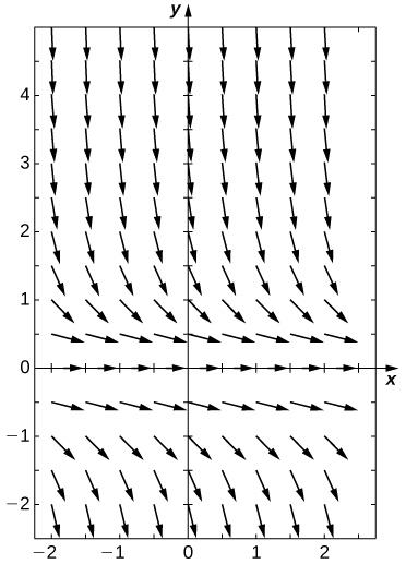
3) \( C=−3\)

4) Solve the logistic equation for \( C=10\) and an initial condition of \( P(0)=2.\)

Answer

\( P=\dfrac{10e^{10x}}{e^{10x}+4}\)

5) Solve the logistic equation for \( C=−10\) and an initial condition of \( P(0)=2\).

6) A population of deer inside a park has a carrying capacity of \( 200\) and a growth rate of \( 2%\). If the initial population is \( 50\) deer, what is the population of deer at any given time?

Answer

\( P(t)=\dfrac{10000e^{0.02t}}{150+50e^{0.02t}}\)

7) A population of frogs in a pond has a growth rate of \( 5%.\) If the initial population is \( 1000\) frogs and the carrying capacity is \( 6000\), what is the population of frogs at any given time?

8) [T] Bacteria grow at a rate of \( 20%\) per hour in a petri dish. If there is initially one bacterium and a carrying capacity of \( 1\) million cells, how long does it take to reach \( 500,000\) cells?

Answer

\( 69\) hours \( 5\) minutes

9) [T] Rabbits in a park have an initial population of \( 10\) and grow at a rate of \( 4%\) per year. If the carrying capacity is \( 500\), at what time does the population reach \( 100\) rabbits?

10) [T] Two monkeys are placed on an island. After \( 5\) years, there are \( 8\) monkeys, and the estimated carrying capacity is \( 25\) monkeys. When does the population of monkeys reach \( 16\) monkeys?

Answer

\( 8\) years \( 11\) months

11) [T] A butterfly sanctuary is built that can hold \( 2000\) butterflies, and \( 400\) butterflies are initially moved in. If after \( 2\) months there are now \( 800\) butterflies, when does the population get to \( 1500\) butterflies?

Logistic Population Model with Depletion

The following problems consider the logistic equation with an added term for depletion, either through death or emigration.

12) [T] The population of trout in a pond is given by \( P'=0.4P\left(1−\dfrac{P}{10000}\right)−400\), where \( 400\) trout are caught per year. Use your calculator or computer software to draw a directional field and draw a few sample solutions. What do you expect for the behavior?

Answer

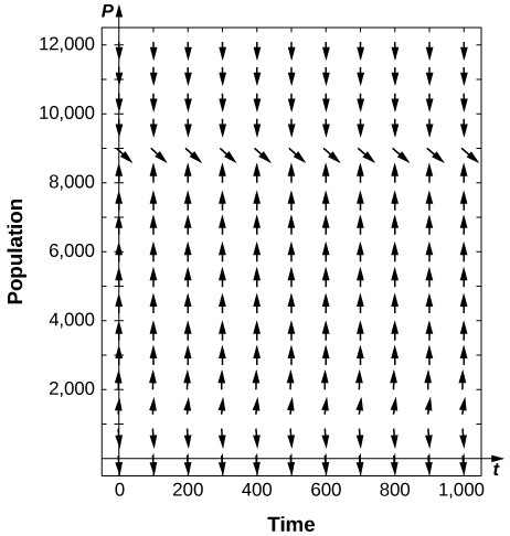
13) In the preceding problem, what are the stabilities of the equilibria \( 0<P_1<P_2\)?

14) [T] For the preceding problem, use software to generate a directional field for the value \( f=400\). What are the stabilities of the equilibria?

Answer

\( P_1\) semi-stable

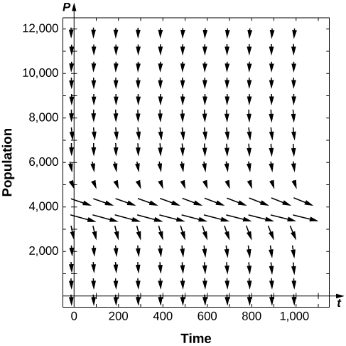
15) [T] For the preceding problems, use software to generate a directional field for the value \( f=600.\) What are the stabilities of the equilibria?

16) [T] For the preceding problems, consider the case where a certain number of fish are added to the pond, or \( f=−200.\) What are the nonnegative equilibria and their stabilities?

Answer

\( P_2>0\) stable

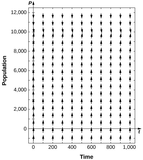
It is more likely that the amount of fishing is governed by the current number of fish present, so instead of a constant number of fish being caught, the rate is proportional to the current number of fish present, with proportionality constant \( k\), as \( P'=0.4P\left(1−\dfrac{P}{10000}\right)−kP.\)

17) [T] For the previous fishing problem, draw a directional field assuming \( k=0.1\). Draw some solutions that exhibit this behavior. What are the equilibria and what are their stabilities?

18) [T] Use software or a calculator to draw directional fields for \( k=0.4\). What are the nonnegative equilibria and their stabilities?

Answer

\( P_1=0\) is semi-stable

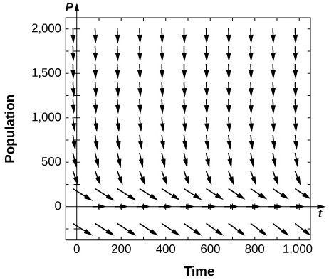
19) [T] Use software or a calculator to draw directional fields for \( k=0.6\). What are the equilibria and their stabilities?

20) Solve this equation, assuming a value of \( k=0.05\) and an initial condition of \( 2000\) fish.

Answer

\( y=\dfrac{−20}{4×10^{−6}−0.002e^{0.01t}}\)

21) Solve this equation, assuming a value of \( k=0.05\) and an initial condition of \( 5000\) fish.

Minimal Sustainable Population Thresholds

The following problems add in a minimal threshold value for the species to survive, \( T\), which changes the differential equation to \( P'(t)=rP\left(1−\dfrac{P}{K}\right)\left(1−\dfrac{T}{P}\right)\).

22) Draw the directional field of the threshold logistic equation, assuming \( K=10,r=0.1,T=2\). When does the population survive? When does it go extinct?

Answer

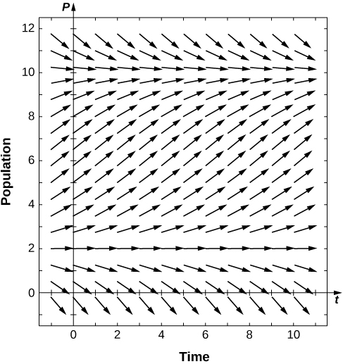
23) For the preceding problem, solve the logistic threshold equation, assuming the initial condition \( P(0)=P_0\).

24) Bengal tigers in a conservation park have a carrying capacity of \( 100\) and need a minimum of \( 10\) to survive. If they grow in population at a rate of \( 1%\) per year, with an initial population of \( 15\) tigers, solve for the number of tigers present.

Answer

\( P(t)=\dfrac{850+500e^{0.009t}}{85+5e^{0.009t}}\)

25) A forest containing ring-tailed lemurs in Madagascar has the potential to support \( 5000\) individuals, and the lemur population grows at a rate of \( 5%\) per year. A minimum of 500 individuals is needed for the lemurs to survive. Given an initial population of \( 600\) lemurs, solve for the population of lemurs.

26) The population of mountain lions in Northern Arizona has an estimated carrying capacity of \( 250\) and grows at a rate of \( 0.25%\) per year and there must be \( 25\) for the population to survive. With an initial population of \( 30\) mountain lions, how many years will it take to get the mountain lions off the endangered species list (at least \( 100\))?

Answer

\( 13\) years months

The Gompertz Equation

The following questions consider the Gompertz equation, a modification for logistic growth, which is often used for modeling cancer growth, specifically the number of tumor cells.

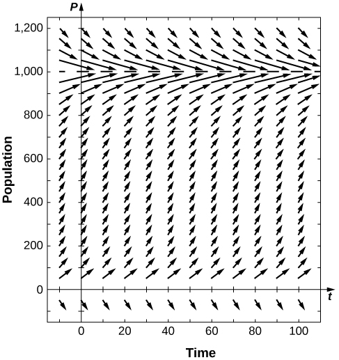
27) The Gompertz equation is given by \( P(t)'=α\ln\left(\frac{K}{P(t)}\right)P(t).\) Draw the directional fields for this equation assuming all parameters are positive, and given that \( K=1.\)

28) Assume that for a population, \( K=1000\) and \( α=0.05\). Draw the directional field associated with this differential equation and draw a few solutions. What is the behavior of the population?

Answer

29) Solve the Gompertz equation for generic \( α\) and \( K\) and \( P(0)=P_0\).

30) [T] The Gompertz equation has been used to model tumor growth in the human body. Starting from one tumor cell on day \( 1\) and assuming \( α=0.1\) and a carrying capacity of \( 10\) million cells, how long does it take to reach “detection” stage at \( 5\) million cells?

Answer

\( 31.465\) days

31) [T] It is estimated that the world human population reached \( 3\) billion people in \( 1959\) and \( 6\) billion in \( 1999\). Assuming a carrying capacity of \( 16\) billion humans, write and solve the differential equation for logistic growth, and determine what year the population reached \( 7\) billion.

32) [T] It is estimated that the world human population reached \( 3\) billion people in \( 1959\) and \( 6\) billion in \( 1999\). Assuming a carrying capacity of \( 16\) billion humans, write and solve the differential equation for Gompertz growth, and determine what year the population reached \( 7\) billion. Was logistic growth or Gompertz growth more accurate, considering world population reached \( 7\) billion on October \( 31,2011?\)

Answer

September \( 2008\)

33) Show that the population grows fastest when it reaches half the carrying capacity for the logistic equation \( P'=rP\left(1−\dfrac{P}{K}\right)\).

34) When does population increase the fastest in the threshold logistic equation \( P'(t)=rP\left(1−\dfrac{P}{K}\right)\left(1−\dfrac{T}{P}\right)\)?

Answer

\( \dfrac{K+T}{2}\)

35) When does population increase the fastest for the Gompertz equation \( P(t)'=α\ln\left(\frac{K}{P(t)}\right)P(t)?\)

Below is a table of the populations of whooping cranes in the wild from \( 1940\) to \( 2000\). The population rebounded from near extinction after conservation efforts began. The following problems consider applying population models to fit the data. Assume a carrying capacity of \( 10,000\) cranes. Fit the data assuming years since \( 1940\) (so your initial population at time \( 0\) would be \( 22\) cranes).

Year (years since conservation began)	Whooping Crane Population
1940(0)	22
1950(10)	31
1960(20)	36
1970(30)	57
1980(40)	91
1990(50)	159
2000(60)	256

Source: www.savingcranes.org/images/...wc_numbers.pdf

36) Find the equation and parameter \( r\) that best fit the data for the logistic equation.

Answer

\( r=0.0405\)

37) Find the equation and parameters \( r\) and \( T\) that best fit the data for the threshold logistic equation.

38) Find the equation and parameter \( α\) that best fit the data for the Gompertz equation.

Answer

\( α=0.0081\)

39) Graph all three solutions and the data on the same graph. Which model appears to be most accurate?

40) Using the three equations found in the previous problems, estimate the population in \( 2010\) (year \( 70\) after conservation). The real population measured at that time was \( 437\). Which model is most accurate?

Answer

Logistic: \( 361\), Threshold: \( 436\), Gompertz: \( 309\).

8.5: First-order Linear Equations

Are the following differential equations linear? Explain your reasoning.

1) \(\displaystyle \frac{dy}{dx}=x^2y+sinx\)

2) \(\displaystyle \frac{dy}{dt}=ty\)

Solution: \(\displaystyle Yes\)

3) \(\displaystyle \frac{dy}{dt}+y^2=x\)

4) \(\displaystyle y'=x^3+e^x\)

Solution: \(\displaystyle Yes\)

5) \(\displaystyle y'=y+e^y\)

Write the following first-order differential equations in standard form.

6) \(\displaystyle y'=x^3y+sinx\)

Solution: \(\displaystyle y'−x^3y=sinx\)

7) \(\displaystyle y'+3y−lnx=0\)

8) \(\displaystyle −xy'=(3x+2)y+xe^x\)

Solution: \(\displaystyle y'+\frac{(3x+2)}{x}y=−e^x\)

9) \(\displaystyle \frac{dy}{dt}=4y+ty+tant\)

10) \(\displaystyle \frac{dy}{dt}=yx(x+1)\)

Solution: \(\displaystyle \frac{dy}{dt}−yx(x+1)=0\)

What are the integrating factors for the following differential equations?

11) \(\displaystyle y'=xy+3\)

12) \(\displaystyle y'+e^xy=sinx\)

Solution: \(\displaystyle e^x\)

13) \(\displaystyle y'=xln(x)y+3x\)

14) \(\displaystyle \frac{dy}{dx}=tanh(x)y+1\)

Solution: \(\displaystyle −ln(coshx)\)

15) \(\displaystyle \frac{dy}{dt}+3ty=e^ty\)

Solve the following differential equations by using integrating factors.

16) \(\displaystyle y'=3y+2\)

Solution: \(\displaystyle y=Ce^{3x}−\frac{2}{3}\)

17) \(\displaystyle y'=2y−x^2\)

18) \(\displaystyle xy'=3y−6x^2\)

Solution: \(\displaystyle y=Cx^3+6x^2\)

19) \(\displaystyle (x+2)y'=3x+y\)

20) \(\displaystyle y'=3x+xy\)

Solution: \(\displaystyle y=Ce^{x^2/2}−3\)

21) \(\displaystyle xy'=x+y\)

22) \(\displaystyle sin(x)y'=y+2x\)

Solution: \(\displaystyle y=Ctan(\frac{x}{2})−2x+4tan(\frac{x}{2})ln(sin(\frac{x}{2}))\)

23) \(\displaystyle y'=y+e^x\)

24) \(\displaystyle xy'=3y+x^2\)

Solution: \(\displaystyle y=Cx^3−x^2\)

25) \(\displaystyle y'+lnx=\frac{y}{x}\)

Solve the following differential equations. Use your calculator to draw a family of solutions. Are there certain initial conditions that change the behavior of the solution?

26) [T] \(\displaystyle (x+2)y'=2y−1\)

Solution: \(\displaystyle y=C(x+2)^2+\frac{1}{2}\)

27) [T] \(\displaystyle y'=3e^{t/3}−2y\)

28) [T] \(\displaystyle xy'+\frac{y}{2}=sin(3t)\)

Solution: \(\displaystyle y=\frac{C}{\sqrt{x}}+2sin(3t)\)

29) [T] \(\displaystyle xy'=2\frac{cosx}{x}−3y\)

30) [T] \(\displaystyle (x+1)y'=3y+x^2+2x+1\)

Solution: \(\displaystyle y=C(x+1)^3−x^2−2x−1\)

31) [T] \(\displaystyle sin(x)y'+cos(x)y=2x\)

32) [T] \(\displaystyle \sqrt{x^2+1}y'=y+2\)

Solution: \(\displaystyle y=Ce^{sinh^{−1}x}−2\)

33) [T] \(\displaystyle x^3y'+2x^2y=x+1\)

Solve the following initial-value problems by using integrating factors.

34) \(\displaystyle y'+y=x,y(0)=3\)

Solution: \(\displaystyle y=x+4e^x−1\)

35) \(\displaystyle y'=y+2x^2,y(0)=0\)

36) \(\displaystyle xy'=y−3x^3,y(1)=0\)

Solution: \(\displaystyle y=−\frac{3x}{2}(x^2−1)\)

37) \(\displaystyle x^2y'=xy−lnx,y(1)=1\)

38) \(\displaystyle (1+x^2)y'=y−1,y(0)=0\)

Solution: \(\displaystyle y=1−e^{tan^{−1}x}\)

39) \(\displaystyle xy'=y+2xlnx,y(1)=5\)

40) \(\displaystyle (2+x)y'=y+2+x,y(0)=0\)

Solution: \(\displaystyle y=(x+2)ln(\frac{x+2}{2})\)

41) \(y'=xy+2xe^x,y(0)=2\)

42) \(\displaystyle \sqrt{x}y'=y+2x,y(0)=1\)

Solution: \(\displaystyle y=2e^{2\sqrt{x}}−2x−2\sqrt{x}−1\)

43) \(\displaystyle y'=2y+xe^x,y(0)=−1\)

Using your expression from the preceding problem, what is the terminal velocity? (Hint: Examine the limiting behavior; does the velocity approach a value?)

44) [T] Using your equation for terminal velocity, solve for the distance fallen. How long does it take to fall \(\displaystyle 5000\) meters if the mass is \(\displaystyle 100\) kilograms, the acceleration due to gravity is \(\displaystyle 9.8\) m/s² and the proportionality constant is \(\displaystyle 4\)?

Solution: \(\displaystyle 40.451\) seconds

45) A more accurate way to describe terminal velocity is that the drag force is proportional to the square of velocity, with a proportionality constant \(\displaystyle k\). Set up the differential equation and solve for the velocity.

46) Using your expression from the preceding problem, what is the terminal velocity? (Hint: Examine the limiting behavior: Does the velocity approach a value?)

Solution: \(\displaystyle \sqrt{\frac{gm}{k}}\)

47) [T] Using your equation for terminal velocity, solve for the distance fallen. How long does it take to fall \(\displaystyle 5000\) meters if the mass is \(\displaystyle 100\) kilograms, the acceleration due to gravity is \(\displaystyle 9.8\)m/s² and the proportionality constant is \(\displaystyle 4\)? Does it take more or less time than your initial estimate?

For the following problems, determine how parameter \(\displaystyle a\) affects the solution.

48) Solve the generic equation \(\displaystyle y'=ax+y\). How does varying \(\displaystyle a\) change the behavior?

Solution: \(\displaystyle y=Ce^x−a(x+1)\)

49) Solve the generic equation \(\displaystyle y'=ax+y.\) How does varying \(\displaystyle a\) change the behavior?

50) Solve the generic equation \(\displaystyle y'=ax+xy\). How does varying \(\displaystyle a\) change the behavior?

Solution: \(\displaystyle y=Ce^{x^2/2}−a\)

51) Solve the generic equation \(\displaystyle y'=x+axy.\) How does varying \(\displaystyle a\) change the behavior?

52) Solve \(\displaystyle y'−y=e^{kt}\) with the initial condition \(\displaystyle y(0)=0\). As \(\displaystyle k\) approaches \(\displaystyle 1\), what happens to your formula?

Solution: \(\displaystyle y=\frac{e^{kt}−e^t}{k−1}\)

Chapter Review Exercise

True or False? Justify your answer with a proof or a counterexample.

1) The differential equation \(\displaystyle y'=3x^2y−cos(x)y''\) is linear.

2) The differential equation \(\displaystyle y'=x−y\) is separable.

Solution: \(\displaystyle F\)

3) You can explicitly solve all first-order differential equations by separation or by the method of integrating factors.

4) You can determine the behavior of all first-order differential equations using directional fields or Euler’s method.

Solution: \(\displaystyle T\)

For the following problems, find the general solution to the differential equations.

5) \(\displaystyle y′=x^2+3e^x−2x\)

6) \(\displaystyle y'=2^x+cos^{−1}x\)

Solution: \(\displaystyle y(x)=\frac{2^x}{ln(2)}+xcos^{−1}x−\sqrt{1−x^2}+C\)

7) \(\displaystyle y'=y(x^2+1)\)

8) \(\displaystyle y'=e^{−y}sinx\)

Solution: \(\displaystyle y(x)=ln(C−cosx)\)

9) \(\displaystyle y'=3x−2y\)

10) \(\displaystyle y'=ylny\)

Solution: \(\displaystyle y(x)=e^{e^{C+x}}\)

For the following problems, find the solution to the initial value problem.

11) \(\displaystyle y'=8x−lnx−3x^4,y(1)=5\)

12) \(\displaystyle y'=3x−cosx+2,y(0)=4\)

Solution: \(\displaystyle y(x)=4+\frac{3}{2}x^2+2x−sinx\)

13) \(\displaystyle xy'=y(x−2),y(1)=3\)

14) \(\displaystyle y'=3y^2(x+cosx),y(0)=−2\)

Solution: \(\displaystyle y(x)=−\frac{2}{1+3(x^2+2sinx)}\)

15) \(\displaystyle (x−1)y'=y−2,y(0)=0\)

16) \(\displaystyle y'=3y−x+6x^2,y(0)=−1\)

Solution: \(\displaystyle y(x)=−2x^2−2x−\frac{1}{3}−\frac{2}{3}e^{3x}\)

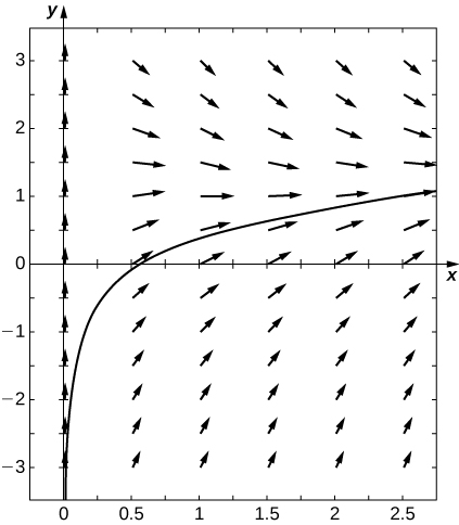
For the following problems, draw the directional field associated with the differential equation, then solve the differential equation. Draw a sample solution on the directional field.

17) \(\displaystyle y'=2y−y^2\)

18) \(\displaystyle y'=\frac{1}{x}+lnx−y,\) for \(\displaystyle x>0\)

Solution: \(\displaystyle y(x)=Ce^{−x}+lnx\)

For the following problems, use Euler’s Method with \(\displaystyle n=5\) steps over the interval \(\displaystyle t=[0,1].\) Then solve the initial-value problem exactly. How close is your Euler’s Method estimate?

19) \(\displaystyle y'=−4yx,y(0)=1\)

20) \(\displaystyle y'=3^x−2y,y(0)=0\)

Solution: Euler: \(\displaystyle 0.6939\), exact solution: \(\displaystyle y(x)=\frac{3^x−e^{−2x}}{2+ln(3)}\)

For the following problems, set up and solve the differential equations.

21) A car drives along a freeway, accelerating according to \(\displaystyle a=5sin(πt),\) where \(\displaystyle t\) represents time in minutes. Find the velocity at any time \(\displaystyle t\), assuming the car starts with an initial speed of \(\displaystyle 60\) mph.

22) You throw a ball of mass \(\displaystyle 2\) kilograms into the air with an upward velocity of \(\displaystyle 8\) m/s. Find exactly the time the ball will remain in the air, assuming that gravity is given by \(\displaystyle g=9.8m/s^2\).

Solution: \(\displaystyle \frac{40}{49}\) second

23) You drop a ball with a mass of \(\displaystyle 5\) kilograms out an airplane window at a height of \(\displaystyle 5000\)m. How long does it take for the ball to reach the ground?

24) You drop the same ball of mass \(\displaystyle 5\) kilograms out of the same airplane window at the same height, except this time you assume a drag force proportional to the ball’s velocity, using a proportionality constant of \(\displaystyle 3\) and the ball reaches terminal velocity. Solve for the distance fallen as a function of time. How long does it take the ball to reach the ground?

Solution: \(\displaystyle x(t)=5000+\frac{245}{9}−\frac{49}{3}t−\frac{245}{9}e^{−5/3t},t=307.8\) seconds

25) A drug is administered to a patient every \(\displaystyle 24\) hours and is cleared at a rate proportional to the amount of drug left in the body, with proportionality constant \(\displaystyle 0.2\). If the patient needs a baseline level of \(\displaystyle 5\) mg to be in the bloodstream at all times, how large should the dose be?

26) A \(\displaystyle 1000\) -liter tank contains pure water and a solution of \(\displaystyle 0.2\) kg salt/L is pumped into the tank at a rate of \(\displaystyle 1\) L/min and is drained at the same rate. Solve for total amount of salt in the tank at time \(\displaystyle t\).

Solution: \(\displaystyle T(t)=200(1−e^{−t/1000})\)

27) You boil water to make tea. When you pour the water into your teapot, the temperature is \(\displaystyle 100°C.\) After \(\displaystyle 5\) minutes in your \(\displaystyle 15°C\) room, the temperature of the tea is \(\displaystyle 85°C\). Solve the equation to determine the temperatures of the tea at time \(\displaystyle t\). How long must you wait until the tea is at a drinkable temperature (\(\displaystyle 72°C\))?

28) The human population (in thousands) of Nevada in \(\displaystyle 1950\) was roughly \(\displaystyle 160\). If the carrying capacity is estimated at \(\displaystyle 10\) million individuals, and assuming a growth rate of \(\displaystyle 2%\) per year, develop a logistic growth model and solve for the population in Nevada at any time (use \(\displaystyle 1950\) as time = 0). What population does your model predict for \(\displaystyle 2000\)? How close is your prediction to the true value of \(\displaystyle 1,998,257\)?

Solution: \(\displaystyle P(t)=\frac{1600000e^{0.02t}}{9840+160e^{0.02t}}\)

Repeat the previous problem but use Gompertz growth model. Which is more accurate?

Contributors and Attributions

• Gilbert Strang (MIT) and Edwin “Jed” Herman (Harvey Mudd) with many contributing authors. This content by OpenStax is licensed with a CC-BY-SA-NC 4.0 license. Download for free at http://cnx.org.