3.5: Implicit Differentiation

In the previous sections we learned to find the derivative, \( \frac{dy}{dx}\), or \(y^\prime \), when \(y\) is given explicitly as a function of \(x\). That is, if we know \(y=f(x)\) for some function \(f\), we can find \(y^\prime \). For example, given \(y=3x^2-7\), we can easily find \(y^\prime =6x\). (Here we explicitly state how \(x\) and \(y\) are related. Knowing \(x\), we can directly find \(y\).)

Sometimes the relationship between \(y\) and \(x\) is not explicit; rather, it is implicit. For instance, we might know that \(x^2-y=4\). This equality defines a relationship between \(x\) and \(y\); if we know \(x\), we could figure out \(y\). Can we still find \(y^\prime \)? In this case, sure; we solve for \(y\) to get \(y=x^2-4\) (hence we now know \(y\) explicitly) and then differentiate to get \(y^\prime =2x\).

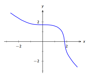
Sometimes the implicit relationship between \(x\) and \(y\) is complicated. Suppose we are given \(\sin(y)+y^3=6-x^3\). A graph of this implicit function is given in Figure 2.19. In this case there is absolutely no way to solve for \(y\) in terms of elementary functions. The surprising thing is, however, that we can still find \(y^\prime \) via a process known as implicit differentiation.

Figure 2.19: A graph of the implicit function \(\sin (y)+y^3=6-x^2\).

Implicit differentiation is a technique based on the Chain Rule that is used to find a derivative when the relationship between the variables is given implicitly rather than explicitly (solved for one variable in terms of the other).

We begin by reviewing the Chain Rule. Let \(f\) and \(g\) be functions of \(x\). Then \[\frac{d}{dx}\Big(f(g(x))\Big) = f^\prime(g(x))\cdot g'(x).\] Suppose now that \(y=g(x)\). We can rewrite the above as

\[\frac{d}{dx}\Big(f(y)\Big) = f^\prime(y)\cdot y^\prime , \quad \text{or}\quad \frac{d}{dx}\Big(f(y)\Big)= f^\prime(y)\cdot \frac{dy}{dx}.\label{2.1}\]

These equations look strange; the key concept to learn here is that we can find \(y^\prime \) even if we don't exactly know how \(y\) and \(x\) relate.

We demonstrate this process in the following example.

Example 67: Using Implicit Differentiation

Find \(y^\prime \) given that \(\sin(y) + y^3=6-x^3\).

Solution

We start by taking the derivative of both sides (thus maintaining the equality.) We have :

\[ \frac{d}{dx}\Big(\sin(y) + y^3\Big)=\frac{d}{dx}\Big(6-x^3\Big).\]

The right hand side is easy; it returns \(-3x^2\).

The left hand side requires more consideration. We take the derivative term--by--term. Using the technique derived from Equation 2.1 above, we can see that \[\frac{d}{dx}\Big(\sin y\Big) = \cos y \cdot y^\prime .\]

We apply the same process to the \(y^3\) term.

\[\frac{d}{dx}\Big(y^3\Big) = \frac{d}{dx}\Big((y)^3\Big) = 3(y)^2\cdot y^\prime .\]

Putting this together with the right hand side, we have

\[\cos(y)y^\prime +3y^2y^\prime = -3x^2.\]

Now solve for \(y^\prime \).

\[\begin{align*} \cos(y)y^\prime +3y^2y^\prime &= -3x^2.\\ \big(\cos y+3y^2\big)y^\prime &= -3x^2\\ y^\prime &= \frac{-3x^2}{\cos y+3y^2} \end{align*}\]

This equation for \(y^\prime \) probably seems unusual for it contains both \(x\) and \(y\) terms. How is it to be used? We'll address that next.

Implicit functions are generally harder to deal with than explicit functions. With an explicit function, given an \(x\) value, we have an explicit formula for computing the corresponding \(y\) value. With an implicit function, one often has to find \(x\) and \(y\) values at the same time that satisfy the equation. It is much easier to demonstrate that a given point satisfies the equation than to actually find such a point.

For instance, we can affirm easily that the point \((\sqrt[3]{6},0)\) lies on the graph of the implicit function \(\sin y + y^3=6-x^3\). Plugging in \(0\) for \(y\), we see the left hand side is \(0\). Setting \(x=\sqrt[3]6\), we see the right hand side is also \(0\); the equation is satisfied. The following example finds the equation of the tangent line to this function at this point.

Example 68: Using Implicit Differentiation to find a tangent line

Find the equation of the line tangent to the curve of the implicitly defined function \(\sin y + y^3=6-x^3\) at the point \((\sqrt[3]6,0)\).

Solution

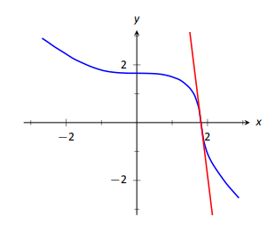
In Example 67 we found that \[y^\prime = \frac{-3x^2}{\cos y +3y^2}.\]We find the slope of the tangent line at the point \((\sqrt[3]6,0)\) by substituting \(\sqrt[3]6\) for \(x\) and \(0\) for \(y\). Thus at the point \((\sqrt[3]6,0)\), we have the slope as \[y^\prime = \frac{-3(\sqrt[3]{6})^2}{\cos 0 + 3\cdot0^2} = \frac{-3\sqrt[3]{36}}{1} \approx -9.91.\]

Therefore the equation of the tangent line to the implicitly defined function \(\sin y + y^3=6-x^3\) at the point \((\sqrt[3]{6},0)\) is \[y = -3\sqrt[3]{36}(x-\sqrt[3]{6})+0 \approx -9.91x+18.\]The curve and this tangent line are shown in Figure 2.20.

Figure 2.20: The function \(\sin y +y^3=6-x^2\) and its tangent line at the point \((\sqrt[3]{6},0)\).

This suggests a general method for implicit differentiation. For the steps below assume \(y\) is a function of \(x\).

1. Take the derivative of each term in the equation. Treat the \(x\) terms like normal. When taking the derivatives of \(y\) terms, the usual rules apply except that, because of the Chain Rule, we need to multiply each term by \(y^\prime \).
2. Get all the \(y^\prime \) terms on one side of the equal sign and put the remaining terms on the other side.
3. Factor out \(y^\prime \); solve for \(y^\prime \) by dividing.

Practical Note: When working by hand, it may be beneficial to use the symbol \(\frac{dy}{dx}\) instead of \(y^\prime \), as the latter can be easily confused for \(y\) or \(y^1\).

Example 69: Using Implicit Differentiation

Given the implicitly defined function \(y^3+x^2y^4=1+2x\), find \(y^\prime \).

Solution

We will take the implicit derivatives term by term. The derivative of \(y^3\) is \(3y^2y^\prime \).

The second term, \(x^2y^4\), is a little tricky. It requires the Product Rule as it is the product of two functions of \(x\): \(x^2\) and \(y^4\). Its derivative is \(x^2(4y^3y^\prime ) + 2xy^4\). The first part of this expression requires a \(y^\prime \) because we are taking the derivative of a \(y\) term. The second part does not require it because we are taking the derivative of \(x^2\).

The derivative of the right hand side is easily found to be \(2\). In all, we get:

\[3y^2y^\prime + 4x^2y^3y^\prime + 2xy^4 = 2.\]

Move terms around so that the left side consists only of the \(y^\prime \) terms and the right side consists of all the other terms:

\[3y^2y^\prime + 4x^2y^3y^\prime = 2-2xy^4.\]

Factor out \(y^\prime \) from the left side and solve to get

\[y^\prime = \frac{2-2xy^4}{3y^2+4x^2y^3}.\]

To confirm the validity of our work, let's find the equation of a tangent line to this function at a point. It is easy to confirm that the point \((0,1)\) lies on the graph of this function. At this point, \(y^\prime = 2/3\). So the equation of the tangent line is \(y = 2/3(x-0)+1\). The function and its tangent line are graphed in Figure 2.21.

Figure 2.21: A graph of the implicitly defined function \(y^3+x^2y^4 = 1+2x\) along with its tangent line at the point \((0,1)\).

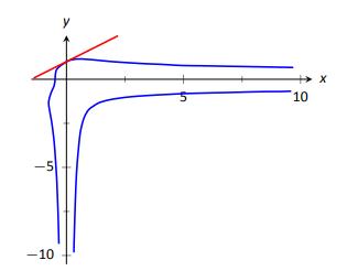
Notice how our function looks much different than other functions we have seen. For one, it fails the vertical line test. Such functions are important in many areas of mathematics, so developing tools to deal with them is also important.

Example 70: Using Implicit Differentiation

Given the implicitly defined function \(\sin(x^2y^2)+y^3=x+y\), find \(y^\prime \).

Solution

Differentiating term by term, we find the most difficulty in the first term. It requires both the Chain and Product Rules.

\[\begin{align*} \frac{d}{dx}\Big(\sin(x^2y^2)\Big) &= \cos(x^2y^2)\cdot\frac{d}{dx}\Big(x^2y^2\Big) \\ &= \cos(x^2y^2)\cdot\big(x^2(2yy^\prime )+2xy^2\big)\\ &= 2(x^2yy^\prime +xy^2)\cos(x^2y^2). \end{align*} \]

We leave the derivatives of the other terms to the reader. After taking the derivatives of both sides, we have

\[2(x^2yy^\prime +xy^2)\cos(x^2y^2) + 3y^2y^\prime = 1 + y^\prime .\]

We now have to be careful to properly solve for \(y^\prime \), particularly because of the product on the left. It is best to multiply out the product. Doing this, we get

\[2x^2y\cos(x^2y^2)y^\prime + 2xy^2\cos(x^2y^2) + 3y^2y^\prime = 1 + y^\prime .\]

From here we can safely move around terms to get the following:

\[2x^2y\cos(x^2y^2)y^\prime + 3y^2y^\prime - y^\prime = 1 - 2xy^2\cos(x^2y^2).\]

Then we can solve for \(y^\prime \) to get

\[y^\prime = \frac{1 - 2xy^2\cos(x^2y^2)}{2x^2y\cos(x^2y^2)+3y^2-1}.\]

A graph of this implicit function is given in Figure 2.22. It is easy to verify that the points \((0,0)\), \((0,1)\) and \((0,-1)\) all lie on the graph. We can find the slopes of the tangent lines at each of these points using our formula for \(y^\prime \).

Figure 2.22: A graph of the implicitly defined function \(\sin (x^2y^2)+y^3=x+y\).

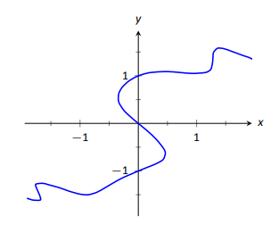
At \((0,0)\), the slope is \(-1\).

At \((0,1)\), the slope is \(1/2\).

At \((0,-1)\), the slope is also \(1/2\).

The tangent lines have been added to the graph of the function in Figure 2.23.

Figure 2.23: A graph of the implicitly defined function \(\sin (x^2y^2)+y^3=x+y\) and certain tangent lines.

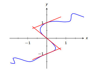
Quite a few "famous'' curves have equations that are given implicitly. We can use implicit differentiation to find the slope at various points on those curves. We investigate two such curves in the next examples.

Example 71: Finding slopes of tangent lines to a circle

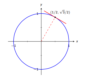
Find the slope of the tangent line to the circle \(x^2+y^2=1\) at the point \((1/2, \sqrt{3}/2)\).

Solution

Taking derivatives, we get \(2x+2yy^\prime =0\). Solving for \(y^\prime \) gives: \[ y^\prime = \frac{-x}{y}.\]

This is a clever formula. Recall that the slope of the line through the origin and the point \((x,y)\) on the circle will be \(y/x\). We have found that the slope of the tangent line to the circle at that point is the opposite reciprocal of \(y/x\), namely, \(-x/y\). Hence these two lines are always perpendicular.

At the point \((1/2, \sqrt{3}/2)\), we have the tangent line's slope as

\[y^\prime = \frac{-1/2}{\sqrt{3}/2} = \frac{-1}{\sqrt{3}} \approx -0.577.\]

A graph of the circle and its tangent line at \((1/2,\sqrt{3}/2)\) is given in Figure 2.24, along with a thin dashed line from the origin that is perpendicular to the tangent line. (It turns out that all normal lines to a circle pass through the center of the circle.)

Figure 2.24: The unit circle with its tangent line at \((1/2,\sqrt{3}/2)\).

This section has shown how to find the derivatives of implicitly defined functions, whose graphs include a wide variety of interesting and unusual shapes. Implicit differentiation can also be used to further our understanding of "regular'' differentiation.

One hole in our current understanding of derivatives is this: what is the derivative of the square root function? That is, \[\frac{d}{dx}\big(\sqrt{x}\big) = \frac{d}{dx}\big(x^{1/2}\big) = \text{?}\]

We allude to a possible solution, as we can write the square root function as a power function with a rational (or, fractional) power. We are then tempted to apply the Power Rule and obtain \[\frac{d}{dx}\big(x^{1/2}\big) = \frac12x^{-1/2} = \frac{1}{2\sqrt{x}}.\]

The trouble with this is that the Power Rule was initially defined only for positive integer powers, \(n>0\). While we did not justify this at the time, generally the Power Rule is proved using something called the Binomial Theorem, which deals only with positive integers. The Quotient Rule allowed us to extend the Power Rule to negative integer powers. Implicit Differentiation allows us to extend the Power Rule to rational powers, as shown below.

Let \(y = x^{m/n}\), where \(m\) and \(n\) are integers with no common factors (so \(m=2\) and \(n=5\) is fine, but \(m=2\) and \(n=4\) is not). We can rewrite this explicit function implicitly as \(y^n = x^m\). Now apply implicit differentiation.

\[\begin{align*}y &= x^{m/n} \\ y^n &= x^m \\ \frac{d}{dx}\big(y^n\big) &= \frac{d}{dx}\big(x^m\big) \\ n\cdot y^{n-1}\cdot y^\prime &= m\cdot x^{m-1} \\ y^\prime &= \frac{m}{n} \frac{x^{m-1}}{y^{n-1}} \quad \text{(now substitute \(x^{m/n}\) for \(y\))} \\ &= \frac{m}{n} \frac{x^{m-1}}{(x^{m/n})^{n-1}} \quad \text{(apply lots of algebra)}\\ &= \frac{m}n x^{(m-n)/n}\\ &= \frac{m}n x^{m/n -1}.\end{align*}\]

The above derivation is the key to the proof extending the Power Rule to rational powers. Using limits, we can extend this once more to include all powers, including irrational (even transcendental!) powers, giving the following theorem.

Theorem 21: Power Rule for Differentiation

Let \(f(x) = x^n\), where \(n\neq 0\) is a real number. Then \(f\) is a differentiable function, and \(f^\prime(x) = n\cdot x^{n-1}\).

This theorem allows us to say the derivative of \(x^\pi\) is \(\pi x^{\pi -1}\).

We now apply this final version of the Power Rule in the next example, the second investigation of a "famous'' curve.

Example 72: Using the Power Rule

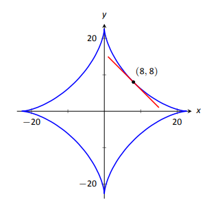
Find the slope of \(x^{2/3}+y^{2/3}=8\) at the point \((8,8)\).

Solution

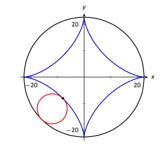
This is a particularly interesting curve called an astroid. It is the shape traced out by a point on the edge of a circle that is rolling around inside of a larger circle, as shown in Figure 2.25.

Figure 2.25: An astroid, traced out by a point on the smaller circle as it rolls inside the larger circle.

To find the slope of the astroid at the point \((8,8)\), we take the derivative implicitly.

\[\begin{align*} \frac23x^{-1/3}+\frac23y^{-1/3}y^\prime &=0\\ \frac23y^{-1/3}y^\prime &= -\frac23x^{-1/3}\\ y^\prime &= -\frac{x^{-1/3}}{y^{-1/3}}\\ y^\prime &= -\frac{y^{1/3}}{x^{1/3}} = -\sqrt[3]{\frac{y}x}. \end{align*}\]

Plugging in \(x=8\) and \(y=8\), we get a slope of \(-1\). The astroid, with its tangent line at \((8,8)\), is shown in Figure 2.26.

Figure 2.26: An astroid with a tangent line.

Implicit Differentiation and the Second Derivative

We can use implicit differentiation to find higher order derivatives. In theory, this is simple: first find \(\frac{dy}{dx}\), then take its derivative with respect to \(x\). In practice, it is not hard, but it often requires a bit of algebra. We demonstrate this in an example.

Example 73: Finding the second derivative

Given \(x^2+y^2=1\), find \(\frac{d^2y}{dx^2} = y^{\prime\prime}\).

Solution

We found that \(y^\prime = \frac{dy}{dx} = -x/y\) in Example 71. To find \(y^{\prime\prime}\), we apply implicit differentiation to \(y^\prime \).

\[\begin{align*} y^{\prime\prime} &= \frac{d}{dx}\big(y^\prime \big) \\ &= \frac{d}{dx}\left(-\frac xy\right)\qquad \text{(Now use the Quotient Rule.)} \\ &= -\frac{y(1) - x(y^\prime )}{y^2} \end{align*}\]

replace \(y^\prime \) with \(-x/y\):

\[\begin{align*}&= -\frac{y-x(-x/y)}{y^2} \\ &= -\frac{y+x^2/y}{y^2}.\end{align*}\]

While this is not a particularly simple expression, it is usable. We can see that \(y^{\prime\prime}>0\) when \(y<0\) and \(y^{\prime\prime}<0\) when \(y>0\). In Section 3.4, we will see how this relates to the shape of the graph.

Logarithmic Differentiation

Consider the function \(y=x^x\); it is graphed in Figure 2.27. It is well--defined for \(x>0\) and we might be interested in finding equations of lines tangent and normal to its graph. How do we take its derivative?

Figure 2.27: A plot of \(y=x^x\).

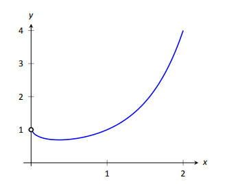
The function is not a power function: it has a "power'' of \(x\), not a constant. It is not an exponential function: it has a "base'' of \(x\), not a constant.

A differentiation technique known as logarithmic differentiation becomes useful here. The basic principle is this: take the natural log of both sides of an equation \(y=f(x)\), then use implicit differentiation to find \(y^\prime \). We demonstrate this in the following example.

Example 74: Using Logarithmic Differentiation

Given \(y=x^x\), use logarithmic differentiation to find \(y^\prime \).

Solution

As suggested above, we start by taking the natural log of both sides then applying implicit differentiation.

\[\begin{align*} y &= x^x \\ \ln (y) &= \ln (x^x) \text{(apply logarithm rule)}\\ \ln (y) &= x\ln x \text{(now use implicit differentiation)}\\ \frac{d}{dx}\Big(\ln (y)\Big) &= \frac{d}{dx}\Big(x\ln x\Big) \\ \frac{y^\prime }{y} &= \ln x + x\cdot\frac1x\\ \frac{y^\prime }{y} &= \ln x + 1\\ y^\prime &= y\big(\ln x+1\big) \text{(substitute \(y=x^x\))}\\ y^\prime &= x^x\big(\ln x+1\big). \end{align*} \]

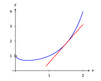
To "test'' our answer, let's use it to find the equation of the tangent line at \(x=1.5\). The point on the graph our tangent line must pass through is \((1.5, 1.5^{1.5}) \approx (1.5, 1.837)\). Using the equation for \(y^\prime \), we find the slope as

\[y^\prime = 1.5^{1.5}\big(\ln 1.5+1\big) \approx 1.837(1.405) \approx 2.582.\]

Thus the equation of the tangent line is \(y = 1.6833(x-1.5)+1.837\). Figure 2.28 graphs \(y=x^x\) along with this tangent line.

Figure 2.22: A graph of \(y=x^x\) and its tangent line at \(x=1.5\).

Implicit differentiation proves to be useful as it allows us to find the instantaneous rates of change of a variety of functions. In particular, it extended the Power Rule to rational exponents, which we then extended to all real numbers. In the next section, implicit differentiation will be used to find the derivatives of inverse functions, such as \(y=\sin^{-1} x\).