3.1: Double and Iterated Integrals Over Rectangles

\[ y=f(x)=e^{-5x^2} , 0\leq x \leq 1\]

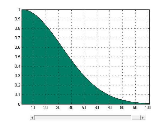
Figure 15.1-0

\[ \int_a^b f(x)\;dx = \lim_{n\rightarrow\infty}\sum_{i=1}^n f(x_i)\, \Delta x_i \]

A fundamental method to calculate the area: the base of function f(x) is equally divide into n pieces whose width are \( \Delta x \). Then \( S=\Delta x f(x_i) \) is the area of the rectangle at the location \(\Delta x_i\) and its height is \(f(x_i)\) among the range \( \Delta x_i\). Through summing all these rectangular pieces together, we can roughly estimate the area under the function \( f(x) \) in its domain. The equation \( \sum_{i=1}^n f(x_i)\, \Delta x_i \) can be used to represent this process.

However, \( \sum_{i=1}^n f(x_i)\, \Delta x_i \) can only help us to estimate the value, which means errors still exist. In this case, limits help us to fix the problem.

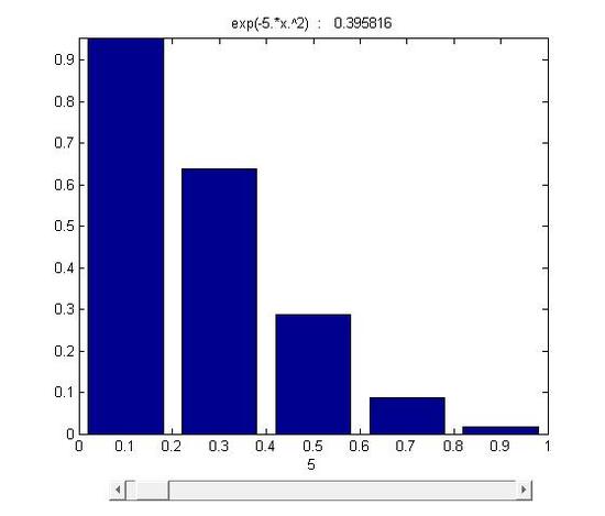
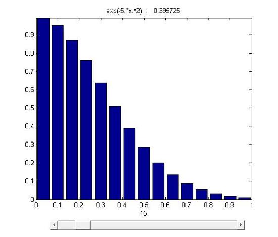
figure 15.1-1

As it was mentioned, the area was divided into n stripes. As \( n \rightarrow \infty \) and \(\Delta x \rightarrow 0\), stripes\( \Delta x f(x_i) \)approachs to a line whose length is equal to the height of \( f(x_i) \). Eventually, through infinite division and accumulation, the error is reduced to zero and the sum of \( f(x) \Delta x\) equals to the area under the curve.

\[ \int_a^b f(x)\;dx = \lim_{n\rightarrow\infty}\sum_{i=1}^n f(x_i)\, \Delta x_i \]

Thus, we can conclude that the integral is the function of accumulation as it accumulates infinite number of strips in a certain domain to calculate the area. Similarly, the double integral is also a function of accumulation. It accumulates infinite number of small 3D strips to calculate the volume of 3D objects.

\[ V=\int \int_R f(x_i,y_i) dx= \lim_{n\rightarrow\infty}\sum_{k=1}^n f(x_i,y_i)\Delta A_i \]

\(R\) is the domain of the function (the area that you want to integrate over)

Explanation:as \(n \rightarrow \infty\), the number of strips goes to infinity, \(\Delta A \rightarrow\infty\), the error of calculation goes to 0 and the accumulation of these infinite strips eventually equals the volume of the objects.

Theoretical discussion with descriptive elaboration

Theorem: Fubini's Theorem (First Form)

If \( f(x,y) \) is contunuous throughout the rectangular region R: \(a\leq x \leq b, c\leq y \leq d,\)

then

\[\int \int_R f(x,y)\Delta A=\int_c^d \int_a^b f(x,y)\Delta x \Delta y= \int_a^b \int_c^d f(x,y)\Delta y \Delta x.\]

Fubini's Theorem is usually used to calculate the volume of three dimensional bodies

Figure 15.1-2

\[ V_i= f(x_i,y_i) \Delta A_i= f(x_i,y_i)\Delta x \Delta y \]

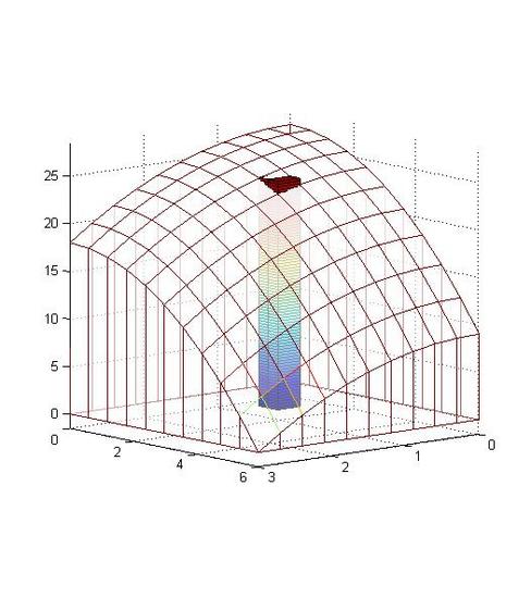
In figure 15.1-2 , \( f(x_i,y_i) \) is the height of the cuboid and \( \Delta A \) is its base. \( V_i \) means that at different location, there is a corresponding cuboid whose height is closed to the average height of the graph at the area \( \Delta A_i \).

Figure 15.1-3

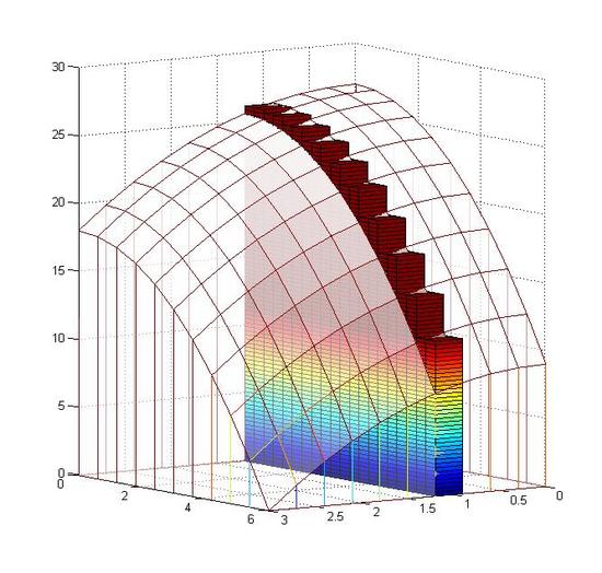
At the specific \( \Delta y_i \), the cuboids with different \(\Delta x_i \) are lined up to form a layer.

Figure 15.1-4

\[ V= \sum_{i=1}^n f(x_i,y_i) \, \Delta A_i=\sum_{i=1}^n f(x_i,y_i)\Delta x_i \Delta y_i \]

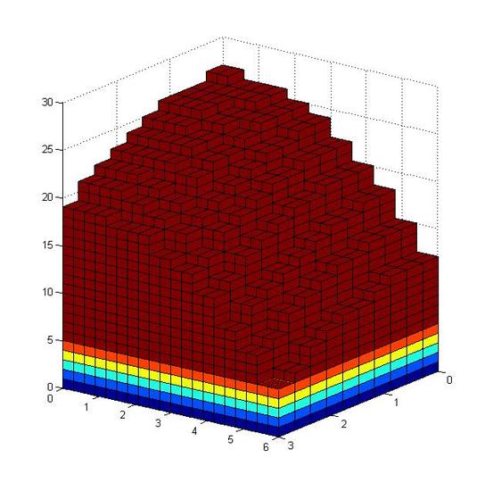
As all the layers are combined together, we get a body that is approximated to the one in the next graph, but the error is still very large.

Figure 15.1-5

\[ V=\lim_{n\rightarrow \infty } \sum_{i=1}^n f(x_i,y_i) \, \Delta A_i \]

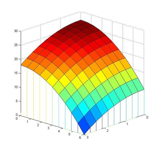
Limit helps to solve this problem. As n goes to infinity, \( \Delta A_i \) becomes smaller eventually turns to a dot. \( f(x_i, y_i) \Delta A_i \) becomes a line and error of volume decreases to zero. Thus, the accumulation of all these lines equal to the volume.

Example 1

Now we can calculate the volume below the function \( f(x,y)=27-x^2-\frac{1}{2}y^2dx dy \) and above \( f(x,y) \), in the domain \( 0\leq x \leq 3 \) and \( 0 \leq y \leq 6 \).

\[\begin{align} & \int_0^6 \int_0^3 27-x^2-\frac{1}{2} y^2dx dy \\ & =\int_0^6 (27-\frac{1}{2}y^2)x-\frac{1}{3}x^3 \Big|_0^3 dy \\ & =\int_0^6 [(27-\frac{1}{2}y^2)\times3-\frac{1}{3}\times 3^3 \\ & =\int_0^6 72-\frac{3}{2}y^2 \ dy \\ & =[72y-\frac{1}{2}y^3]\Big|_0^6 \\ & = (72\times 6-\frac{1}{2}\times6^3)-(0-0) \\ & = 324 \end{align}\]

Figure: (left) from step 1 to step 3 (right) from step 3 to step 6

Example 2

Another way to calculate the volume of the graph:

\[\begin{align} &\int_0^3 \int_0^6 27-x^2-\frac{1}{2} y^2dy dx \\ & = \int_0^3 (27-x^2)y-\frac{1}{6}y^3 \Big|_0^6 \ dx \\ & =\int_0^3 [(27-x^2)\times 6 -\frac{1}{6}\times6^3]-[0-0]\ dx \\ & =\int_0^3 126-6x^2\ dx \\ & = [126x-2x^3]\Big|_0^3 \\ & = (126\times3-2\times 3^3 )-(0-0) \\ & = 324. \end{align}\]

Reminder: the positions of \( \Delta x \) and \( \Delta y \) are different. So are the positions of their domains.

Example 3

Find the volume that is bounded above by the surface \(z=f(x,y)=x^2+y^2\) and below by a rectangule R: \(0\leq x \leq 2, 0\leq y \leq 3 \).

\[\begin{align} & \int_0^2 \int_0^3 x^2+y^2 dy dx \\ & =\int_0^2 x^2y+\frac{1}{3}y^3 \Big|_0^3 dx \\ & =\int_0^2 3x^2+9 dx \\ & =x^3+9x\Big|_0^2 \\ & =(8+18)-0 \\ & =26 \end{align}\]

Contributors and Attributions

Integrated by Justin Marshall.