3.3: Double Integrals Over General Regions

In Section 15.1, we notice that all bases of the objects are rectangular. In 15.2, the area under these objects are nonrectangular. However, the method of accumulation still works.

Introduction

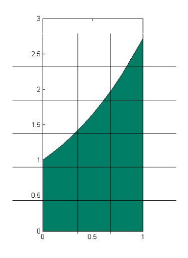
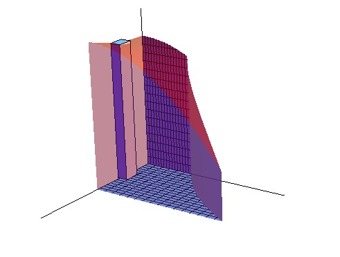
In the Figure \(\PageIndex{1}\), the green figures are the base of the 3D object on the left. Its base is encloesd by \( y=e^x\), \(y=0\), \(x=0\) and \(x=1\), and it was divided into small diamonds. As \(n\), the number of these diamonds, goes to infinity and \( \Delta A= \Delta x \Delta y \) goes to zero, the area of each diamond approximates to a single point, which reduces the estimation error to zero. Thus, through accumulating all these single points, we can calculate the area accurately.

Figure \(\PageIndex{1}\)

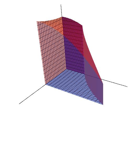
\[ S=\lim_{n\rightarrow \infty}\sum_{k=1}^{n}\Delta A= \iint_R dA \nonumber \]

Theorem: Fubini's Theorem (Stronger Form)

Let \( f(x,y) \) be continuous on a region \(R\).

1. If R is defined by \( a \leq x \leq b, g(x_1) \leq y \leq g(x_2)\), with \(g_1\) and \(g_2\) continous on \([a,b]\), then

\[ \iint_R f(x,y) dA = \int_a^b \int_{g_1(x)}^{g_2(x)} f(x,y)\, dy\, dx \nonumber \]

2. If R is defined by \( c \leq y \leq d, h_1(y) \leq y \leq h_2(y)\), with \(h_1\) and \(h_2\) continous on [c,d], then

\[ \iint_R f(x,y) dA = \int_c^d \int_{h_1(y)}^{h_2(y)} f(x,y) \,dx \,dy \nonumber \]

Fubini's Theorem is usually used to calculate the volume of the objects that have nonrectangule bases.

Figure \(\PageIndex{1}\): Paste Caption Here

Just like the sample in 15.1, \( V_i = f(x,y)\Delta A \) is the volume of the cuboid at a specific location. This cuboid has the height \(f(x,y) \)that is decided by its location. As n, the number of cuboids, goes to infinity, the shape of each cuboid approaches to a line whose height equal to \( f(x_i,y_i) \) and error approaches to zero. Through accumulating infinity number of these "lines", we can accurately calculate the volume of the object.

\[ V=\lim_{n\rightarrow \infty} \sum_{k=1}^{n} f(x_i,y_i)\Delta x \Delta y = \int \int _R f(x,y)\,dA \nonumber \]

Example \(\PageIndex{1}\)

Now, lets calculate the volume under the surface \( f(x,y)=10+x^2-y^2 \) whose domain is enclosed by \(y=e^x\), \(y=0\), \(x=0\) and \(x=1\).

Figure \(\PageIndex{3}\)

\[\begin{align*} \int_0^1 \int_{y=0}^{y=e^x} 10+x^2-y^2 dy dx &= \int_0^1 (10+x^2)y-\frac{1}{3}y^3 \Big|_{y=0}^{y=e^x} dx \\ &= \int_0^1 (10+x^2)e^x-\frac{1}{3}(e^x)^3 dx \\ &= 10e^x +(x^2 e^x-2xe^x+2e^x)-\frac{1}{9}(e^x)^3 \Big |_0^1 \\ &= [10e+(e-2e+2e) - \frac{1}{9}e^3]-[10+(0-0+2)-\frac{1}{9}] \\ &= 11e -\frac{1}{9} e^3 + \frac{107}{9} \end{align*} \]

Example \(\PageIndex{2}\)

Figure \(\PageIndex{3}\)

\[\begin{align*} f(x,y)&=\int_{0}^{1}\int_{y=x^2}^{y=1} 1 dydx \\ &= \int_{0}^{1} y \Big|_{x^2}^{1} dx \\ &=\int_{0}^{1} 1-x^2 dx \\ &= x-\dfrac{1}{3}x^3 \Big|_0^1 \\ &= \dfrac{2}{3} \end{align*} \]

Reverse the order of integration of the function \[f(x,y)=\int_{0}^{1}\int_{y=x^2}^{y=1}1dydx \nonumber \]

Figure \(\PageIndex{4}\)

\[\begin{align*} &=\int_{y=1}^{y=0}\int_{x=0}^{x=\sqrt{y}}1 \; dx dy \\ & =\int_{0}^{1} \sqrt{y} \; dy \\ &= \dfrac{2}{3} y^{\frac{3}{2}} \Big|_{0}^{1} \\ &= \dfrac{2}{3} \end{align*} \]

Reminder:

1. As the equation is transformed, the domains of x and y are also transformed.
2. When \( f(x,y)=1 \), the value of double integral numerically equals to the area of its base.
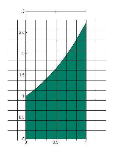
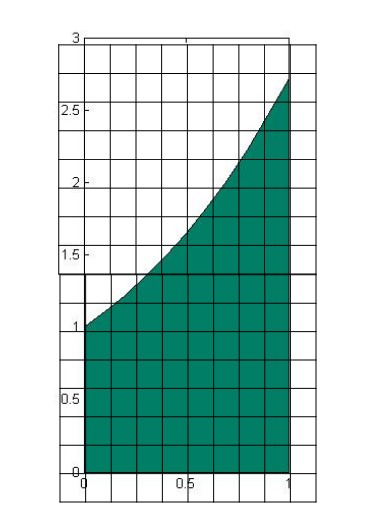
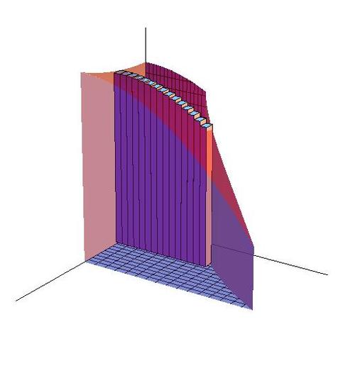
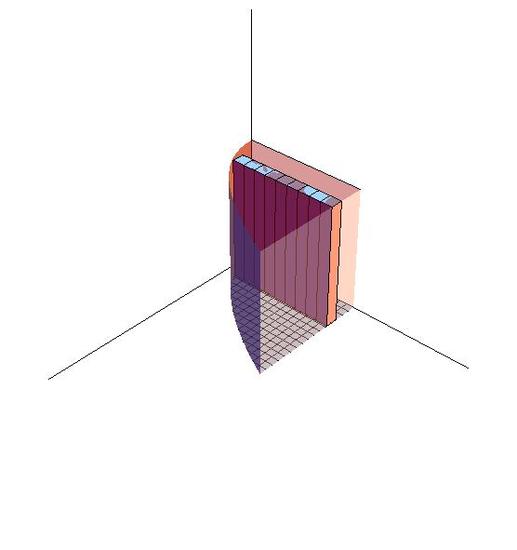
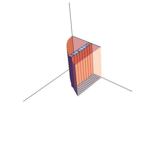
3. The order of \(dx\) and \(dy\) decides the order of accumulation. In figure 15.2-3, stripes are arranged along y axis to form layers and then we can calculate the volume thorough adding all the layers. That's why the function is written as \( \int \int_R f(x,y)dydx\). Similarly, in the Figure 15.2-4, stripes are arranged along x axis to form layers, so the order of dy and dx is switched. That is \( \iint_R f(x,y)dx dy \).

Example \(\PageIndex{5}\)

Calculate the volume above \(f(x，y)=0 \) and \(f(x,y)=1\) in the domain enclosed by \(x=\tan^{-1}(y)\), \(x=0\), \(y=0\) and \(y= 1\).

\[\begin{align*} f(x,y)&= \int_0^1 \int_{x=0}^{x=\tan^{-1}(y) }1 \ dx \ dy \\ &= \int_0^1 \int_{x=0}^{x=\tan^{-1}(y)} 1\ dx \ dy \\ &= \int_0^1 x \Big|_0^{\tan^{-1}} \ dy \\ &= \int_0^1 \tan^{-1}y \ dy \end{align*} \]

In this case, the question become too complicated to be solved. Thus, we need to transform this equation.

\[\begin{align*} f(x,y) &= \int_{x=0}^{x=\tan^{-1} (y)} 1 \; dx \;dy \\ &= \int_{0}^{\frac{\pi}{4}} x \Big|_{\tan (x)}^1 \;dx \\ &= \int_{0}^{\frac{\pi}{4}} (1-\tan (x)) dx \\ &= x+ \ln (\cos (x)) \Big|_0^{\frac{\pi}{4}} \\ &= (\dfrac{\pi}{4} + \ln (\dfrac{\sqrt{2}}{2}) -(0+ \ln 1) \\ &= \dfrac{\pi}{4} \ln (\dfrac{\sqrt{2}}{2}) \end{align*} \]

• Integrated by Justin Marshall.