3.4: Double Integrals in Polar Form
- Page ID
- 580
\( \newcommand{\vecs}[1]{\overset { \scriptstyle \rightharpoonup} {\mathbf{#1}} } \)
\( \newcommand{\vecd}[1]{\overset{-\!-\!\rightharpoonup}{\vphantom{a}\smash {#1}}} \)
\( \newcommand{\dsum}{\displaystyle\sum\limits} \)
\( \newcommand{\dint}{\displaystyle\int\limits} \)
\( \newcommand{\dlim}{\displaystyle\lim\limits} \)
\( \newcommand{\id}{\mathrm{id}}\) \( \newcommand{\Span}{\mathrm{span}}\)
( \newcommand{\kernel}{\mathrm{null}\,}\) \( \newcommand{\range}{\mathrm{range}\,}\)
\( \newcommand{\RealPart}{\mathrm{Re}}\) \( \newcommand{\ImaginaryPart}{\mathrm{Im}}\)
\( \newcommand{\Argument}{\mathrm{Arg}}\) \( \newcommand{\norm}[1]{\| #1 \|}\)
\( \newcommand{\inner}[2]{\langle #1, #2 \rangle}\)
\( \newcommand{\Span}{\mathrm{span}}\)
\( \newcommand{\id}{\mathrm{id}}\)
\( \newcommand{\Span}{\mathrm{span}}\)
\( \newcommand{\kernel}{\mathrm{null}\,}\)
\( \newcommand{\range}{\mathrm{range}\,}\)
\( \newcommand{\RealPart}{\mathrm{Re}}\)
\( \newcommand{\ImaginaryPart}{\mathrm{Im}}\)
\( \newcommand{\Argument}{\mathrm{Arg}}\)
\( \newcommand{\norm}[1]{\| #1 \|}\)
\( \newcommand{\inner}[2]{\langle #1, #2 \rangle}\)
\( \newcommand{\Span}{\mathrm{span}}\) \( \newcommand{\AA}{\unicode[.8,0]{x212B}}\)
\( \newcommand{\vectorA}[1]{\vec{#1}} % arrow\)
\( \newcommand{\vectorAt}[1]{\vec{\text{#1}}} % arrow\)
\( \newcommand{\vectorB}[1]{\overset { \scriptstyle \rightharpoonup} {\mathbf{#1}} } \)
\( \newcommand{\vectorC}[1]{\textbf{#1}} \)
\( \newcommand{\vectorD}[1]{\overrightarrow{#1}} \)
\( \newcommand{\vectorDt}[1]{\overrightarrow{\text{#1}}} \)
\( \newcommand{\vectE}[1]{\overset{-\!-\!\rightharpoonup}{\vphantom{a}\smash{\mathbf {#1}}}} \)
\( \newcommand{\vecs}[1]{\overset { \scriptstyle \rightharpoonup} {\mathbf{#1}} } \)
\(\newcommand{\longvect}{\overrightarrow}\)
\( \newcommand{\vecd}[1]{\overset{-\!-\!\rightharpoonup}{\vphantom{a}\smash {#1}}} \)
\(\newcommand{\avec}{\mathbf a}\) \(\newcommand{\bvec}{\mathbf b}\) \(\newcommand{\cvec}{\mathbf c}\) \(\newcommand{\dvec}{\mathbf d}\) \(\newcommand{\dtil}{\widetilde{\mathbf d}}\) \(\newcommand{\evec}{\mathbf e}\) \(\newcommand{\fvec}{\mathbf f}\) \(\newcommand{\nvec}{\mathbf n}\) \(\newcommand{\pvec}{\mathbf p}\) \(\newcommand{\qvec}{\mathbf q}\) \(\newcommand{\svec}{\mathbf s}\) \(\newcommand{\tvec}{\mathbf t}\) \(\newcommand{\uvec}{\mathbf u}\) \(\newcommand{\vvec}{\mathbf v}\) \(\newcommand{\wvec}{\mathbf w}\) \(\newcommand{\xvec}{\mathbf x}\) \(\newcommand{\yvec}{\mathbf y}\) \(\newcommand{\zvec}{\mathbf z}\) \(\newcommand{\rvec}{\mathbf r}\) \(\newcommand{\mvec}{\mathbf m}\) \(\newcommand{\zerovec}{\mathbf 0}\) \(\newcommand{\onevec}{\mathbf 1}\) \(\newcommand{\real}{\mathbb R}\) \(\newcommand{\twovec}[2]{\left[\begin{array}{r}#1 \\ #2 \end{array}\right]}\) \(\newcommand{\ctwovec}[2]{\left[\begin{array}{c}#1 \\ #2 \end{array}\right]}\) \(\newcommand{\threevec}[3]{\left[\begin{array}{r}#1 \\ #2 \\ #3 \end{array}\right]}\) \(\newcommand{\cthreevec}[3]{\left[\begin{array}{c}#1 \\ #2 \\ #3 \end{array}\right]}\) \(\newcommand{\fourvec}[4]{\left[\begin{array}{r}#1 \\ #2 \\ #3 \\ #4 \end{array}\right]}\) \(\newcommand{\cfourvec}[4]{\left[\begin{array}{c}#1 \\ #2 \\ #3 \\ #4 \end{array}\right]}\) \(\newcommand{\fivevec}[5]{\left[\begin{array}{r}#1 \\ #2 \\ #3 \\ #4 \\ #5 \\ \end{array}\right]}\) \(\newcommand{\cfivevec}[5]{\left[\begin{array}{c}#1 \\ #2 \\ #3 \\ #4 \\ #5 \\ \end{array}\right]}\) \(\newcommand{\mattwo}[4]{\left[\begin{array}{rr}#1 \amp #2 \\ #3 \amp #4 \\ \end{array}\right]}\) \(\newcommand{\laspan}[1]{\text{Span}\{#1\}}\) \(\newcommand{\bcal}{\cal B}\) \(\newcommand{\ccal}{\cal C}\) \(\newcommand{\scal}{\cal S}\) \(\newcommand{\wcal}{\cal W}\) \(\newcommand{\ecal}{\cal E}\) \(\newcommand{\coords}[2]{\left\{#1\right\}_{#2}}\) \(\newcommand{\gray}[1]{\color{gray}{#1}}\) \(\newcommand{\lgray}[1]{\color{lightgray}{#1}}\) \(\newcommand{\rank}{\operatorname{rank}}\) \(\newcommand{\row}{\text{Row}}\) \(\newcommand{\col}{\text{Col}}\) \(\renewcommand{\row}{\text{Row}}\) \(\newcommand{\nul}{\text{Nul}}\) \(\newcommand{\var}{\text{Var}}\) \(\newcommand{\corr}{\text{corr}}\) \(\newcommand{\len}[1]{\left|#1\right|}\) \(\newcommand{\bbar}{\overline{\bvec}}\) \(\newcommand{\bhat}{\widehat{\bvec}}\) \(\newcommand{\bperp}{\bvec^\perp}\) \(\newcommand{\xhat}{\widehat{\xvec}}\) \(\newcommand{\vhat}{\widehat{\vvec}}\) \(\newcommand{\uhat}{\widehat{\uvec}}\) \(\newcommand{\what}{\widehat{\wvec}}\) \(\newcommand{\Sighat}{\widehat{\Sigma}}\) \(\newcommand{\lt}{<}\) \(\newcommand{\gt}{>}\) \(\newcommand{\amp}{&}\) \(\definecolor{fillinmathshade}{gray}{0.9}\)Up until now, we have dealt with double integrals in the Cartesian coordinate system. This is helpful in situations where the domain can be expressed simply in terms of \(x\) and \(y\). However, many problems are not so easy to graph. If the domain has the characteristics of a circle or cardioid, then it is much easier to solve the integral using polar coordinates.
Introduction
The Cartesian system focuses on navigating to a specific point based on its distance from the x, y, and sometimes z axes. In polar form, there are generally two parameters for navigating to a point: \(r\) and \( \theta \). \(r\) represents the magnitude of the vector that stretches from the origin to the desired point. In other words, \(r\) is the distance directly to that coordinate point. \( \theta \) represents the angle that the aforementioned theoretical vector would make with the x-axis. This creates a circular type of motion as we adjust the value of \( \theta \), which allows us to express a circle of radius 1 as \( r = 1 \) as opposed to \( x^2 + y^2 = 1 \) in Cartesian coordinates.
Polar Double Integration Formula
Many of the double integrals that we have encountered so far have involved circles or at least expressions with \(x^2 + y^2\). When we see these expressions a bell should ring and we should shout, "Can't we use polar coordinates." The answer is, "Yes" but only with care. Recall that when we changed variables in single variable integration such as \(u = 2x\), we needed to work out the stretching factor \(du = 2dx\). The idea is similar with two variable integration. When we change to polar coordinates, there will also be a stretching factor. This is evident \since the area of the "polar rec\tangle" is not just as one may expect. The picture is shown below.
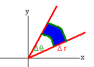
Even if \( \Delta{r}\) and \( \Delta{q}\) are very small, the area is not the product \( \Delta{r}\, \Delta{q} \). This comes from the definition of radians. An arc that extends \( \Delta{q}\) radians a distance \(r\) out from the origin has length\( r\, \Delta{q}\). If both \(\Delta r\) and \(\Delta q\) are very small then the polar rectangle has area
\[ Area = r \Delta{r} \Delta{q}. \nonumber \]
This leads us to the following theorem
Let \(f(x,y)\) be a continuous function defined over a region \(R\) bounded in polar coordinates by
\( r_1(q) < r < r_2(q) \) and \( q_1 < q < q_2 \).
Then
\[ \iint_R f(x,y)\,dy\,dx =\int_{\theta_1}^{\theta_2} \int_{r_1(\theta)}^{r_2(\theta)} f(r\cos \theta,r\sin \theta)\,r\,dr\,d\theta.\nonumber \]
Notice the extra "\(r\)" in the theorem
Theoretical discussion with descriptive elaboration
The area of a closed and bounded region \(r\) in the polar coordinate plane is given by
\[ A = \iint_{R}^{ }\ r \, dr\, d \theta. \nonumber \]
To find the bounds for a domain in this form, we use a similar technique as with integrals in rectangular form. Beginning at the origin with \(r = 0 \) we increase the value of \(r\) until we find the maximum and minimum overall distance from the origin. Similarly, for \(\theta \) we start at \( \theta = 0 \) and find the minimum and maximum angles that the domain makes with the orgin. The maximum distance away from the origin and the maximum angle with the origin that defines the boundary represents the upper bound for the double integral. The minimum distance and the minimum angle with the origin makes the lower bound for the double integral.
For example, to find the bounds for \(r\), we look to see what the minimum and maximum overall distances from the origin are in terms of \(r\). Sometimes problems will explicitly give you the curves that form the domain, other times you may need to look at a graph to determine the domain. Regardless, if the origin is contained in the domain, then the lower bound for \(r\) will be 0. The upper bound will be whatever curve encompasses the rest of the domain.
\( \theta \) is usually simpler to compute. The lower and upper bounds are the minimum and maximum angles that the domain makes with the origin. Trigonometric functions can be used to determine the extreme angles that the function makes with the origin.
If an equation is provided, it is helpful to use the conversions:
\[ x = r\, \cos \,\theta\nonumber \]
\[y = r\, \sin \,\theta \nonumber \]
to convert equations from Cartesian to polar form. If one must determine the bounds from a provided graph, it can be helpful to guess and check by plotting some test points to see if your bounds truly match the provided graph.
If you need to convert an integral from Cartesian to polar form, graph the domain using the Cartesian bounds and your knowledge of curves in the Cartesian domain. Then use the method described above to derive the bounds in polar form. Once the integral is set up, it may be solved exactly like an integral using rectangular coordinates.
Find the volume to the part of the paraboloid
\[ z = 9 - x^2 - y^2 \nonumber \]
that lies inside the cylinder
\[ x^2 + y^2 = 4. \nonumber \]
Solution
The surfaces are shown below.
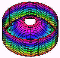
This is definitely a case for polar coordinates. The region \(R\) is the part of the xy-plane that is inside the cylinder. In polar coordinates, the cylinder has equation
\[ r^2 = 4. \nonumber \]
Taking square roots and recalling that \(r\) is positive gives
\[ r = 2. \nonumber \]
The inside of the cylinder is thus the polar rectangle
\( 0 < r < 2 \) \( 0 < q < 2\pi\).
The equation of the parabola becomes
\[ z = 9 - r^2. \nonumber \]
We find the integral
\[ \int _0^{2\pi}\int_0^2 \left(9-r^2\right) r\,dr\,d\theta.\nonumber \]
This integral is a matter of routine and evaluates to \( 28\pi\).
Find the volume of the part of the sphere of radius 3 that is left after drilling a cylindrical hole of radius 2 through the center.
Solution
The picture is shown below
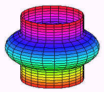
The region this time is the annulus (washer) between the circles \(r = 2\) and \(r = 3\) as shown below.
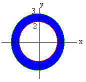
The sphere has equation
\[ x^2 + y^2 + z^2 = 9 .\nonumber \]
In polar coordinates this reduces to
\[ r^2 + z^2 = 9. \nonumber \]
Solving for \(z\) by subtracting \(r^2\) and taking a square root we get top and bottom surfaces of
\[z=\sqrt{9-r^2} \;\;\; \text{and} \;\;\; z=-\sqrt{9-r^2}. \nonumber \]
We get the double integral
\[\int_0^{2\pi} \int_2^3 (\sqrt{9-r^2}+ \sqrt{9-r^2})r\; dr d\theta. \nonumber \]
This integral can be solved by letting
\[u = 9 - r^2 \;\;\; \text{and} \;\;\;du = -2r\,dr.\nonumber \]
After substituting we get
\[\begin{align*} &-\dfrac{1}{2}\int_{0}^{2\pi}\int_{5}^{0} 2u^{\frac{1}{2}} \; du d\theta \\ &= -\dfrac{2}{3}\int_{0}^{2\pi}[u^{\frac{3}{2}}]_5^0 \; d\theta \\ &= \dfrac{20 \sqrt{5} \pi}{3}.\end{align*} \]
Change the Cartesian integral into an equivalent polar integral, then solve it.
\[ \int_{1}^{\sqrt{3}}\int_{1}^{x}dydx \nonumber \]
Solution
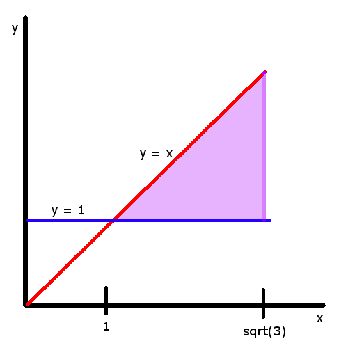
The point at (\(\sqrt{3}\), 1) is at an angle of \(\pi/6\) from the origin. The point at (\(\sqrt{3}, \sqrt{3}\) is at an angle of \(\pi/4\) from the origin. In terms of \(r\), the domain is bounded by two equations \(r=csc\theta\) and \(r=\sqrt{3}\sec\theta\). Thus, the converted integral is
\[ \int_{csc\theta}^{\sqrt{3}\sec\theta}\int_{\pi/6}^{\pi/4}rdrd\theta. \nonumber \]
Now the integral can be solved just like any other integral.
\[\begin{align*} &\int_{\pi/6}^{\pi/4} \int_{csc\theta}^{\sqrt{3}\sec\theta}rdrd\theta \\ & =\int_{\pi/6}^{\pi/4} (\dfrac{3}{2} \sec^2\theta - \dfrac{1}{2} \csc^2\theta) d\theta \\ & = \left [ \dfrac{3}{2} \tan\theta + \dfrac{1}{2}\cot\theta \right ] _{\dfrac{\pi}{6}}^{\dfrac{\pi}{4}} \\ & =2 - \sqrt{3}. \end{align*}\nonumber \]
Find the area of the region cut from the first quadrant by the curve \( r = \sqrt{2 - \sin2\theta}\).
Solution
Note that it is not even necessary to draw the region in this case because all of the information needed is already provided. Because the region is in the first quadrant, the domain is bounded by \( \theta = 0 \) and \( \theta = \dfrac{\pi}{2} \). The sole boundary for \(r\) is \(r = \sqrt{2 - \sin2\theta}\) so the integral is
\[\begin{align*} & \int_{0}^{\pi/2}\int_{0}^{\sqrt{2 - \sin2\theta}} rdrd\theta \\ &= \int_{0}^{\pi/2} \left [ \dfrac{r^2}{2} \right ] _{0}^{\sqrt{2 - \sin2\theta}} d\theta \\ &= \int_{0}^{\pi/2} \dfrac{2 - \sin2\theta}{2} d\theta \\ &= \int_{0}^{\pi/2} 1 - \dfrac{\sin2\theta}{2} d\theta \\ &= \left [ \theta + \dfrac{\cos2\theta}{4} \right ] _{0}^{\pi/2} \\ &= \dfrac{\pi}{2} - \dfrac{1}{4}. \end{align*}\nonumber \]
Contributors and Attributions
- Michael Rea (UCD), Larry Green
Integrated by Justin Marshall.


